11.4: Astrophysical Black Holes

Learning Objectives

• Explain the following laws within the Ideal Gas Law

What Do You Think: Detecting Black Holes

So far we have discussed black holes from a theoretical perspective. But how do we know that any of this has a basis in reality? How can we even begin to study objects that emit no light and are more massive than the Sun? For a long time the answer was, “we can’t.” That began to change several decades ago when advances in astronomical instruments opened new vistas on the Universe. Black holes popped out, sometimes glowing brightly in the darkness, other times remaining hidden except for their influence on visible neighbors. In this section we look at how black holes are detected and how they affect the Universe and its contents.

Stellar Mass Black Holes

The first observational evidence that black holes are more than mere theoretical oddities was obtained using instruments borne aloft by sounding rockets in the 1960s. The rocket payloads were simple and small, and the flights were short, lasting just long enough to carry their loads above the atmosphere before falling back to Earth. Nonetheless, these flights were a critical demonstration that astrophysical x-ray sources exist.

Without going above the atmosphere it is impossible to know if x-ray sources are in the sky. The atmosphere is completely opaque to x-rays and higher energy photons. Sounding rocket flights proved that x-ray sources are present, but they gave only short views of those sources. The situation improved with the launch of the first orbiting x-ray telescope, Uhuru, in late 1970.

Uhuru takes its name from the Swahili for “freedom,” a reference to the location of its launch platform in Kenya. It was the first of a series of three similar satellites launched by NASA in the 1970s. Uhuru was a survey instrument, and it provided a view of the sky very different from sounding rockets. The rocket flights were short and their instruments primitive. Because their detectors were only able to view the sky for the few minutes that the rocket payload was above the atmosphere, only a small number of very bright sources were detected. Most astronomers of the time did not expect an x-ray telescope to see much more than this. They were wrong.

Over its three-year lifetime, Uhuru cataloged more than 300 x-ray sources spread over the entire sky. That does not sound like a lot when compared to the thousands of stars visible to even the naked eye, but it was only a start. Subsequent x-ray missions have cataloged more than 100,000 sources. We now know that many of these sources are black holes, but the evidence for that was decades building.

One of the most interesting sources observed with Uhuru was a very bright source called Cygnus X-1 (see Figure 11.11), so designated because it is the brightest x-ray source in the constellation Cygnus. The source had been discovered nearly a decade earlier and tentatively identified with a blue supergiant star. The improved x-ray observations possible with Uhuru showed that the source varied extremely rapidly, up to several times each second. The variations set limits on the size of the emitting region because any source can only vary as quickly as light can travel across it. In this case it could be no bigger than about a quarter of the Earth–Moon distance. See Going Further 11.4: Light Travel Time and Variability.

The identification of the blue supergiant with the x-ray source was strengthened as additional observations of the source were made in various wave bands. But blue supergiants do not emit x-rays in the amounts detectable from Earth. That suggested the supergiant had a companion, invisible in optical light, which was responsible for the x-rays. Careful study of the supergiant’s spectrum revealed that it was indeed a member of a binary system; the star’s spectral lines were seen to shift back and forth with a period of about five and a half days. These motions placed constraints on the mass of the unseen companion, requiring it to be at least 10 solar masses. A massive invisible companion that is a powerful x-ray emitter suggests the presence of a black hole, and the evidence for a black hole has slowly increased over the subsequent four decades.

Figure 11.11: The optical image on the left shows the region of the galaxy containing Cygnus X-1 (red box). The x-ray image on the right was taken by the Chandra X-ray Observatory. Credit: Optical (Digitized Sky Survey); x-ray (NASA/CXC)

GOING FURTHER 11.4: LIGHT TRAVEL TIME AND VARIABILITY

Cygnus X-1 belongs to a class of objects called high-mass x-ray binaries. In these systems, a massive normal star orbits a compact object, usually a neutron star or black hole. Rarely, the compact object is a white dwarf. White dwarfs, neutron stars, and (stellar mass) black holes are the remnants left over when stars have died. The x-rays are produced when the compact companion captures some of the wind produced by the normal star. Very massive stars like blue supergiants have powerful stellar winds, amounting to the loss of perhaps 10 solar masses every million years. This rate is about a billion times larger than the mass lost by the Sun due to the solar wind.

The material captured from the stellar wind forms an accretion disk around the compact object and spirals down into it. The gravitational energy lost during the accretion process is enough to heat the gas in the accretion disk to millions or even tens of millions of kelvin. At those temperatures, much hotter than the surface of even the hottest normal star, the disk glows in x-rays. There can also be secondary x-ray emission from the surface of the star facing the disk. As x-rays from the disk heat the stellar photosphere, they cause it to also glow in x-rays.

The x-ray emission from high-mass x-ray binaries looks essentially the same whether the accretion is onto a neutron star or a black hole. It is usually necessary to make a careful study of the motion of the normal star in order to distinguish between the two. Black holes are more massive than neutron stars, and so they affect the motion of the companion to a larger degree than a neutron star. Once the motion of the star is known, and the mass of the compact object has been determined, scientists can deduce whether the invisible component is a black hole or a neutron star: the upper limit for the mass of a neutron star is about three times the mass of the Sun. Thus, if the accreting object is larger than about three solar masses, it is likely to be a black hole. In the case of Cygnus X-1, the black hole mass is determined to be about 15 solar masses.

In addition to high-mass x-ray binaries, there are low-mass x-ray binaries. In these systems a normal star, typically with a mass similar to that of the Sun, orbits a massive compact object, either a neutron star or a black hole. Occasionally a white dwarf is present in these systems instead of a normal star. Material is transferred from the star to its compact companion. Essentially, material on the surface of the normal star will find itself equally attracted by the gravity of the normal star and the compact object. It can thus fall off the normal star onto its companion. This will only happen if the separation between the two is quite small.

As the material is transferred it forms an accretion disk, allowing it to shed angular momentum and thus fall into the compact object. Just as in high-mass x-ray binaries, the accretion disk is heated to millions of kelvin by the release of gravitational energy, and thus it glows in x-rays. Figure 11.12 shows several artistic renderings of x-ray binary systems. X-ray binaries are also sometimes sources of gamma-rays and radio waves.

Figure 11.12: X-ray binary systems are systems in which a normal star orbits a neutron star or black hole. These artist’s renderings depict two examples of such systems. In the first, at left, a massive star orbits a black hole. In the other system a low-mass star orbits a black hole. If the star and black hole are close enough to each other, then some of the material of the normal star can fall onto the black hole, forming an accretion disk that is hot enough to glow brightly in x-rays, giving the systems their name. Credit: NASA/SSU/Aurore Simonnet

We have suggested that the energy needed to power the x-ray emission from x-ray binary systems comes from the release of gravitational energy. The energy is released as material falls onto the compact object from its companion. But is this a reasonable model for the emission? We have learned enough gravitational physics in the past several chapters that we can answer that question.

Recall that the gravitational potential energy of an object of mass \(m\) in the potential of another object of mass \(M\) a distance \(r\) away is given by

\[PE=-\frac{GMm}{r} \nonumber \]

This says that the energy is proportional to the product of the masses and inversely proportional to the distance between them. The power produced, or luminosity is the energy emitted per unit time. We can compare this to the observed luminosity of x-ray binary systems. The luminosity that might be produced from gravitational potential energy is therefore:

\[L=\frac{\Delta PE}{\Delta t} \nonumber \]

where \(\Delta t\) is the time interval and \(\Delta PE\) is the energy emitted over the time interval. If this power is produced by mass accretion then we can write the following:

\[L=\frac{\Delta PE}{\Delta t} =−\left (\frac{GM}{r} \right )\left( \frac{\Delta m}{\Delta t}\right ) \nonumber \]

We are assuming that the mass (M) of the accreting object, the black hole in this case, is not changed appreciably by the mass \(\Delta m\) falling onto it over the time interval \(\Delta t\). Under this assumption, the only thing changing on the right side of the equation is the mass being lost by the companion star and attracted by the black hole; this is the accretion rate, Δm/Δt. Recall that the minus sign in the equation for potential energy is just a convention in the definition.

Accretion Rate and Luminosity

The luminosity of x-ray binaries ranges from about 10²⁶ W to 10³¹ W, or from about one solar luminosity to 100,000 solar luminosities. In this activity we see how to use these numbers to test the feasibility of the mass accretion model for x-ray binaries.

Worked Examples:

1. Find the accretion rate for a black hole emitting 10²⁶ W of luminosity.

Given:

• luminosity \(L = 10^{26}\, {\rm W}\)
• gravitational constant: \(G = 6.67\times 10^{-11}\, {\rm N m^2\,/ \, kg^2}\)
• mass of black hole: \(M = 15M_{Sun} = 3\times 10^{31}\, {\rm kg}\)
• speed of light: \(c = 3\times 10^8\, {\rm m/s}\)

Find: Δm/Δt, the accretion rate in units of kg/s

• Concept(s):

  \(L=−\left ( \dfrac{GM}{r}\right ) \left ( \dfrac{Δm}{Δt}\right ) \)

  and r is the Schwarzschild radius,

  \(R_{Sch}=\dfrac{2GM}{c^2}\)

Solution:

• We can rearrange the equation in terms of \(\frac{\Delta m}{\Delta t}\), substitute the Schwarzschild radius for r, and then plug in the appropriate numbers.
  First solve for \(\frac{\Delta m}{\Delta t}\) by multiplying by \(-\frac{r}{GM}\).

  \(\dfrac{\Delta m}{\Delta t} = -\dfrac{Lr}{GM}\)

  Now substitute \(R_{Sch}\) for the radius, \(r\):

  \(\dfrac{\Delta m}{\Delta t} = - \dfrac{L}{\cancel {GM}} \cdot \dfrac{2\cancel{GM}}{c^2}= -\dfrac{2L}{c^2}\)

Notice that the mass of the black hole cancels. Only the power emitted matters.

\(\dfrac{\Delta m}{\Delta t} = - \dfrac{2L}{c^2} = -2\left [\dfrac{10^{26}\, {\rm W}}{(3\times 10^8\,{\rm m/s})^2}\right ] = -2.29 \times 10^9\,{\rm kg/s}\)

2. Express the accretion rate in terms of solar masses.

Converting units,

\( (-2.29\times 10^9\, {\rm \cancel{kg}/\cancel{s}})(1 M_{Sun}\, / \, 2\times 10^{30}\, {\rm \cancel{kg}})(3.15\times 10^7\,{\rm \cancel{s}}\, / \, 1\, {\rm yr})=-3.5\times 10^{-14}\,M_{Sun}/{\rm yr}\)

This is a very small amount of mass to transfer. For the higher luminosity systems, the accretion rate would be about a hundred thousand times larger, but it is still very small and not a challenge for these systems. The mass model for X-ray binaries seems quite reasonable, at least from these simple energy arguments.

As an aside, the final value for Δm/Δt is negative because the star that the black hole is accreting matter from is losing mass. When this negative quantity is multiplied by the minus sign in the original equation for luminosity, we see that luminosity is a positive quantity, as it should be.

Questions

1.

2.

Notice from the last activity that the mass of the black hole does not affect the accretion rate. If we drop a given amount of mass from a great distance onto any black hole, we will get the same luminosity out. Can you think of a reason why? We will look at this process in more detail in the next section.

Supermassive Black Holes

Active galactic nuclei (AGN) are another class of bright x-ray sources. They are found in active galaxies, naturally. Only a few percent of galaxies are active. AGN are bright sources of radio and gamma-ray emission as well as x-rays. Optically, AGN are usually not very impressive, being well below the threshold of detection by the unaided eye. In fact, even the brightest optical AGN are barely visible with the aid of a small telescope. This is due to the fact that all AGN are very far away.

Various types of active galaxies are shown in Figure 11.13.

Figure 11.13: AGN are seen in various wave bands: (a) the radio galaxy Cygnus A, (b) the galaxy M87 as seen in optical light, and (c) the Seyfert galaxy NGC 1275 as seen in gamma-rays. AGN are seen at various distances and with varying energy outputs. Credit: (a) Image courtesy of NRAO/AUI, (b) NASA and The Hubble Heritage Team (STScI/AURA), (c) NASA/DOE/Fermi LAT Collaboration

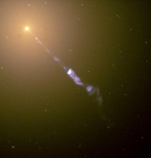
It turns out that most AGN lie at immense distances, hundreds of millions or even billions of light-years from the Milky Way. From that perspective it is clear that their luminosities must be enormous. In fact, the brightest AGN in the sky put out the energy of billions, or sometimes trillions, of Suns, comparable to or even exceeding the brightness of a large galaxy like the Milky Way. Even more impressive is that these luminosities are seen across the entire spectrum, from radio up through infrared and optical, all the way to x-rays and gamma-rays: comparable amounts of energy are seen in each of these wave bands, see Figure 11.14. Something interesting is going on in AGN.

Figure 11.14: AGN emit tremendous energy all across the electromagnetic spectrum. The two-humped shape is common to all AGN, but notice that the energy being emitted extends across ~20 orders of magnitude. Credit: NASA/SSU/Carolyn Peruta

AGN are not just immensely bright, their brightness can vary on extremely short timescales (see Figure 11.15). Fluctuations range from seconds, minutes, or hours to months or years. Typically the longer the time for the variation the larger the AGN is. Some AGN change their brightness by a factor of a hundred over roughly year-long timescales, but the shorter fluctuations are the interesting ones for our purposes. They set upper limits to the size of the emitting region. These fluctuations suggest that the emitting region of AGN is no more than a few light-hours across, a size comparable to the region of our Solar System occupied by the gas giant planets. The shortest timescales for changes in AGN brightness are thought to be caused by emission processes in powerful relativistic jets ejected from their cores. These do not place any constraints on the size of the total emission region.

Figure 11.15: The brightness of AGN varies with time. The variations are seen on timescales as short as milliseconds and as long as years. Light travel time allows us to estimate the size of the emitting region. Credit: NASA/SSU/Aurore Simonnet

In the 1960s, when AGN were first beginning to be understood, astronomers were faced with a seemingly unsolvable puzzle. How was it possible to explain the energetics of a region comparable in size to the solar system that exceeded the energy output of an entire galaxy? These regions were always seen in the very centers of large galaxies. Sometimes they glowed brightly across the entire electromagnetic spectrum, but sometimes they would shine only in radio, or just in optical. As x-ray astronomy developed in the 1970s and afterward, it became clear many of the brightest x-ray sources were associated with AGN. How to explain these weird objects?

By a process of elimination, the idea of accretion onto a black hole was fairly quickly deemed the most likely explanation. Thus, AGN became some of the earliest evidence for the reality of black holes, just around the time when x-ray binaries did as well. The following activity, similar to the previous example on the energetics of x-ray binaries, shows why this accretion model was deemed feasible.

Accretion Onto a Supermassive Black Hole

Worked Example:

1. Assume that AGN are powered by accretion onto a black hole. The black holes at the centers of galaxies are likely to be larger than the ones found in stellar binary systems, but as we showed earlier, the mass of the black hole does not matter. Estimate the accretion rate required to produce a luminosity of 10¹² solar luminosities. First find the rate in units of kg/s and then convert to M_Sun/yr.

• Given: A luminosity \(10^{12}\) times larger than the Sun which has a luminosity of \(4\times 10^{26}\, {\rm W} \rightarrow L = 4\times 10^{38}\, {\rm W}\)
• Find: Δm/Δt, the accretion rate in units of kg/s and M_Sun/yr
• Concept(s): \(\frac{\Delta m}{\Delta t} = -\frac{2L}{c^2}\)
  where the speed of light , \(c = 3\times 10^8\,{\rm m/s}\)
• Solution:
  \(\dfrac{\Delta m}{\Delta t} = -2 \left ( \dfrac{4\times 10^{38}\,{\rm W}}{(3\times 10^8\,{\rm m/s})^2}\right ) = -8.9\times 10^{21}\,{\rm kg/s}\)

Converting to solar masses per year:

\((-8.9\times 10^{21}\,{\rm \cancel{kg}/\cancel{s}})(1\,M_{Sun}\,/\,2\times 10^{30}\,{\rm \cancel{kg}})(3.15\times 10^7\,{\rm \cancel{s}}\,/\,{\rm yr}) = -0.16 \,M_{Sun}\,/\,{\rm yr}\)

You should have found a much larger accretion rate is required to produce the typical bright AGN luminosities, a trillion times the previous one. At this rate, the black hole must devour about one solar mass every six years. That is quite a lot. It is too much for a small black hole to consume, and in any event , any black hole that feeds at such a prodigious rate cannot stay small for long.

Questions

1.

The unifed model of AGN, depicted in Figure 11.16, explains how AGN are powered— by an accretion disk surrounding a supermassive black hole. As with accretion disks around forming stars, the accretion disks around supermassive black holes also have jets of material beaming out. The next activity will lead you through how the very different looking observations of active galaxies can all be explained by this single model.

Figure 11.16: This artist’s conception illustrates the unified model for AGN. Astronomers have found that all large galaxies contain supermassive black holes in their centers, with masses of millions or billions of solar masses. If material is falling into these black holes, then the nucleus is said to be active. It glows brightly from radio to gamma-ray energies, in some cases dominating the emission from the galaxy by a factor of one hundred. The detailed workings of AGN are still not understood. Credit: NASA/SSU/Aurore Simonnet

THE UNIFIED AGN MODEL

Watch the movie and then answer the questions.

VIEW TRANSCRIPT

1. 2. 3. 4. 5.

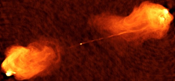
Figure 11.17 shows the AGN Centaurus A in several different wave bands. Each wave band reveals different aspects of the galaxy’s structure.

Figure 11.17: This image gives an example of the active galaxy Centaurus A as seen in x-ray, optical, and radio emission. Each wave band reveals different aspects of the galaxy’s structure. About a percent of galaxies seem to be active at any given time, but there is evidence that all galaxies go through an active phase at some point (or points) in their evolution. Credit: x-ray (NASA/CXC/M. Karovska et al. http://chandra.harvard.edu/photo/2002/0157/); optical (Digitized Sky Survey U.K. Schmidt Image/STScI); radio continuum image (NRAO/VLA/J. Condon et al.); radio 21-cm image (NRAO/VLA/J.Van Gorkom/Schminovich et al.).

Under the assumption that AGN are powered by accretion onto a black hole, we have found that higher accretion rates are needed for a higher luminosity. But how do we know that the highest accretion rates correspond to the most massive black holes? We might intuitively expect this to be the case since it is easier to collect more material through a large event horizon than through a small one. The surface area of a black hole event horizon depends on its radius squared, so that means it depends on the square of the black hole mass as well. Since more massive black holes have much larger event horizons, we expect that they could support higher accretion rates. While this argument is sensible, it is not very quantitative. How much mass should we expect to be able to fall into a black hole of a given size?

The answer to this question was first explored by Arthur Eddington in a very different context. Eddington was the same British astrophysicist who measured the bending of starlight around the Sun during the eclipse of 1919. Eddington’s approach was slightly different from what we have outlined above. He did not consider the size of the black hole event horizon—in fact, he was not thinking about black holes at all. He was thinking about the stability of the most massive stars, and he compared the inward pull of gravity to the outward force of radiation pressure felt by the material in the stars’ atmospheres. Eddington reasoned that radiation pressure must act on the gas , and the higher a star’s luminosity, the higher the outward pressure on the gas. Eventually, if the luminosity were large enough, the outgoing radiation would push on the material in the atmosphere hard enough to overcome gravity, blasting it off the star. In essence, he said that at the point where the luminosity is so great that radiation pressure cancels gravity, the star would become unbound; radiation will blow it apart.

The same argument can be applied to accreting black holes. As the accretion rate increases, so does the luminosity. As the luminosity increases, the radiation pressure it exerts on the in-falling material also rises. If the luminosity becomes large enough—as the result of a large accretion rate—then it will be able to halt the accretion. There should therefore be an upper limit to the amount of material that can fall onto a black hole, a limit imposed by the very radiation produced by the gravitational energy released through accretion.

This limiting value for the luminosity is now called the Eddington limit or Eddington luminosity. It has the value

\(L_{edd}=6.3\,M_{BH}\)

where L_edd is the luminosity in W, M_BH is mass of the black hole in kg, and the constant 6.31 has units of W/kg. The expression gives the highest accretion rate possible for a spherically accreting object. The Eddington luminosity is proportional to the mass, which means that the higher the mass, the higher the maximum luminosity. See Going Further 11.5: Derivation of the Eddington Luminosity to see how we arrive at this expression.

Eddington Luminosity

Use the Eddington Luminosity Tool to find the maximum luminosity for several black hole masses.

1.

2.

3.

4.

We do not expect spherical accretion onto a black hole, we expect it to be via an accretion disc. As a result, the Eddington luminosity is really just a guide. We can use it to give us an idea of how the accretion onto a black hole is related to its mass, but there could be (and probably are) large variations among different black hole accretion systems.

GOING FURTHER 11.5: DERIVATION OF THE EDDINGTON LUMINOSITY

Energy arguments suggest strongly that the gravity of black holes provides the power for AGN. However, these arguments are not completely convincing. After all, it could be that some other undiscovered object or process is powering AGN. In the last decade any such doubts have been mostly set aside. Careful studies of the motions of visible material near AGN have shown that a black hole lies at their core. One of the strongest cases for the AGN-black hole connection is the nearby weak AGN, NGC 4258, also called M106 (Figure 11.18). The motion of gas in the galactic nucleus indicates the presence of an unseen 40 million solar mass object within 0.1 parsecs of the center— the typical distance between stars in the vicinity of the Sun is roughly one parsec. So we have about one solar mass of material per cubic parsec in our region of the Galaxy. This stands in contrast to 40 million solar masses in 0.001 cubic parsecs in the nucleus of NGC 4258.

Figure 11.18: Analysis of the gas motions in the center of the nearby AGN NGC 4258 indicates the presence of a central object with the mass of 40 million Suns. Top: the area within 0.5 light-years of the black hole is a warped disk. Bottom left: the rotation curve of material near the black hole. Bottom right: An expanded view of NGC 4258. Credit: NASA/SSU/Aurore Simonnet, based on an image by L. Greenhill courtesy of NRAO/AUI.

In addition to detecting the presence of black holes in galaxies, astronomers have also started to determine properties other than mass for some of them. One of these properties is spin. The spin can be deduced by examining emission spectra produced in the accretion disk. For instance, in the active galaxy NGC 1365, astronomers used two x-ray telescopes to measure the spectrum of the material in the accretion disk (Figure 11.19). The XMM-Newton telescope measured the spectrum between 3 and 10 keV. At these energies interpretation of the spectrum is ambiguous because its shape could be the result of either the black hole spin or the presence of obscuring clouds in our line of sight. However, the NuSTAR telescope was able to measure the spectrum out to 79 keV. With this higher energy part of the spectrum, the ambiguity drops away, and only a spinning black hole remains consistent with all the observations, including both of these x-ray observations and other observations at infrared and optical energies.

The black hole at the center of NGC 1365 is observed to be spinning almost as fast as general relativity predicts a black hole should be able to spin. This has important implications for the formation of supermassive black holes, and by extension, for galaxies themselves.

Figure 11.19: The plot at the top shows the x-ray spectra of NGC 1365 from two telescopes, XMM-Newton and NuSTAR. Combining the spectra allows astronomers to test models for the formation of the emission spectrum, one based upon the presence of absorbing clouds in our line of sight, the other based upon the spin of the supermassive black hole in the center of the galaxy. Only the spinning black hole model is consistent with the observations. The bottom image shows the effects of black hole rotation on theoretical energy distributions. Credit: Risaliti, G., et al. (2013), Nature, 494, 449; NASA/JPL-Caltech

Detecting the Milky Way Black Hole

Currently, the strongest observational case for the presence of a supermassive black hole is not in AGN at all. It is in the center of our own Galaxy, the Milky Way. Research carried out by teams at UCLA and at the Max Planck Institute for Astrophysics, near Munich, Germany, have shown that the center of our Galaxy contains a black hole with the mass of four million Suns. This conclusion is the result of watching stars move in the central region. They are seen to be orbiting a massive, invisible object.

Figure 11.20 shows a series of observations of our Galactic center by a team at UCLA led by Andrea Ghez (Figure 11.21). The UCLA team used the Keck Telescope, one of the largest telescopes in the world, located atop the Mauna Kea volcano on the Big Island of Hawaii. The blobs of light in Figure 11.20 are images of stars near the center of our Galaxy, and the dots show the measured positions of several of those stars during almost two decade of observations, from 1995 to 2012. You can see that these stars are all orbiting the same unseen object. That is the location of the black hole at the center of the Milky Way. Figure 11.22 shows an animated version of the data.

Figure 11.20: The orbits of stars within the central 1.0 × 1.0 arcseconds of our Galaxy. While every star in this image has been seen to move over the past 17 years, estimates of orbital parameters are only possible for the eight stars that are closest to the black hole. The annual average positions for these eight stars are plotted as colored dots, which have increasing color saturation with time. Also plotted are the best fitting simultaneous orbital paths. These orbits provide the best evidence yet for a supermassive black hole, which has a mass of 4 million times the mass of the Sun. Credit: Keck/UCLA Galactic Center Group

Figure 11.21: The UCLA Galactic Center Group, led by Andrea Ghez (lower right). For more information, visit the group’s website: http://www.astro.ucla.edu/~ghezgroup/gc/. Credit: Mary Watkins

Figure 11.22: Images taken by Andrea Ghez and her group using the Keck telescope are used to track specific stars orbiting the black hole at the center of the Milky Way. These orbits, and a simple application of Kepler's laws, provide the best evidence yet for a supermassive black hole, which has a mass of 4 million times the mass of the Sun. Especially important are the stars S0-2, which has an orbital period of only 15.78 years, and S0-16, which passes a mere 90 AU from the black hole. Credit: Keck/UCLA Galactic Center Group

Orbits are the key to measuring the masses of astronomical objects. If we want to measure the mass of something, we need to find one or more objects that orbit it and measure the properties of those orbits. Once we know the orbital period and average orbital distance of an orbiting object, we can use that information to measure the force of gravity needed to hold that object in orbit. Then, from the force of gravity, we can determine the total amount of mass in the system, because gravity is directly related to mass.

Consequences of all three of Kepler’s laws of orbital motion are evident in the image and animated image. The orbits of stars around the black hole are ellipses (Kepler’s first law). The stars move faster when they are close to the black hole and slower when they are farther away (Kepler’s second law). Finally, stars orbiting at greater distances have longer orbital periods (Kepler’s third law).

Newton’s version of Kepler’s third law relates the orbital distance, a, and orbital period, p, to the total amount of mass in the system.

\[M=\frac{a^3}{p^2} \nonumber \]

Here M is in units of solar masses, a is in AU, and p is in years. It is easy to see how this formula works for the Earth–Sun system. Plugging in a = 1 AU and p = 1 year gives a total mass for the Earth–Sun system of 1 M_Sun, and you would get the same mass by plugging a and p for any of the other planets. If we apply the formula to the stars in the center of the galaxy, using AU for their orbital sizes and years for their periods, then they determine the mass of the central black hole in terms of solar masses.

By determining the orbital distances and orbital periods of the stars near the Milky Way’s central black hole in this way, the UCLA group reports a mass for the black hole of 4.1 ± 0.4 × 10⁶ M_Sun.

In addition to these stellar motions, evidence for our Galaxy’s supermassive black hole comes from radio emission and occasional x-ray flares. Presumably these happen when gas falls into the black hole.

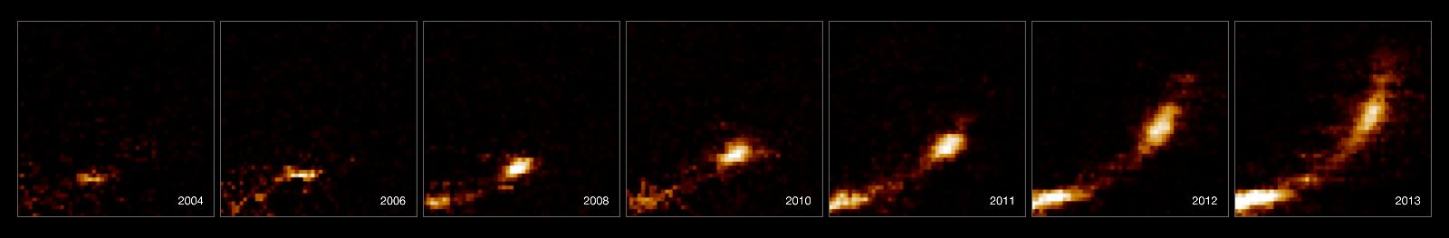
In near infrared wavelengths, ESO's Very Large Telescope (VLT) has observed a gas cloud being tidally stretched (spaghettifiied) by the Milky Way’s black hole. Figure 11.23 is a series of images taken by the VLT from 2004 to 2013. The horizontal axis shows the stretching of the head vs. the tail of the cloud over time and the vertical axis shows how the spread in the velocity of the material has increased over time. The closest approach of the cloud to the black hole is about 25 billion km (about 170 AU).

Figure 11.23: Images taken by the VLT from the years 2004 through 2013 of a cloud near the galactic center. The cloud is being ripped apart by the Milky Way’s central black hole. The horizontal axis in the figure shows the size of the cloud; it has stretched more than 160 billion km. The vertical axis shows velocity; the head of the cloud is moving millions of km/h faster than the tail. The cloud is moving at nearly 1% of the speed of light. Credit: ESO/S. Gillessen

Our galaxy definitely does not host an AGN, though it does host a gigantic black hole in its center, just as do AGN. Why the difference? The answer seems to be the environment of the black hole. In galaxies with large amounts of gas in their centers, the black holes induce AGN behavior as the gas falls into them, releasing vast amounts of gravitational potential energy. In most galaxies, including ours, the galactic nuclei are mainly devoid of gas. Since there is no material falling into the black hole there is no energy released and therefore no AGN.

The fraction of galaxies that exhibit AGN behavior is only around a percent or so at the present time. The proportion is observed to have been larger in the past, and it seems that the AGN phenomenon is related to galactic formation and evolution.

Intermediate Mass Black Holes

So far in this section we have described black holes with masses comparable to stars. These are called stellar mass black holes. We have also discussed the supermassive black holes found in the centers of galaxies. Supermassive black holes are immense, with masses measured in the millions or billions of solar masses, while stellar mass black holes are no larger than about a dozen, or maybe a few dozen, times the mass of the Sun. But what about black holes with masses in the middle? Have astrophysicists found any so-called intermediate mass black holes? The answer, somewhat surprisingly at first, seems to be “maybe.” There is some evidence for these objects, but the evidence is not conclusive.

If we consider how black holes form and grow, we might set aside our initial surprise at the absence of any with intermediate mass. The masses of these black holes would range from several hundred to perhaps tens of thousands of solar masses. What objects would form a black hole of that size?

Stars do not seem able to produce black holes of intermediate sizes. The largest stars are around 200 solar masses, at least in the present-day Universe. But such stars have enormous winds. Their winds allow them to lose most of their mass over their lifetimes. When they eventually do undergo collapse to a black hole, the remnants they leave are in the stellar mass range, measured in tens of solar masses.

We know that most stars are formed in groups, and perhaps these groups could form many massive stars. These would in turn create many stellar mass black holes. Then perhaps these stellar mass black holes could somehow combine to form a single black hole with a mass of a few hundred solar masses, or even a few thousand.

While this scenario seems reasonable, it must not be very common, simply because astronomers do not see very many intermediate mass black holes. In fact, there is debate about whether any have been detected at all. A few candidate objects have been detected via their x-ray emission. These ultra-luminous x-ray sources are brighter than even the brightest x-ray binaries by a factor of ten or so. Some astronomers think that the extra x-ray luminosity is the result of accretion onto a large black hole. Several models have been developed along these lines. None have been completely successful.

Additional evidence for intermediate mass black holes could come from their gravitational effects on stars and gas near to them. That is how the presence of the black holes in the center of the Milky Way and other galaxies has been uncovered. However, intermediate mass black holes have weaker gravity than the supermassive black holes at the centers of galaxies. So they would have a much smaller effect on objects close to them. Detecting any motions they might induce in nearby objects stretches the capabilities of the largest ground-based telescopes, like those used to study the Milky Way center. Even the Hubble Space Telescope is not quite up to the task. Perhaps later generations of telescopes and detectors will be powerful enough to look for the tell-tale signs of distant black holes too small to provide the gravitational wallop of their supermassive cousins.

There is another possibility. Perhaps the merger of stellar mass black holes to form intermediate mass black holes is one step on the way to creating the supermassive black holes we detect. After all, we have seen that only a short time is required (on relevant timescales) to grow a black hole to an extremely large size if material is present to accrete onto it. If this is the correct description, then the reason we do not see many intermediate mass black holes anymore is that they have all been merged into the monsters in galactic centers. This could be part of the normal processes in the early Universe that formed the galaxies or their building blocks.

However, if intermediate mass black holes are still being created in star forming regions, then they should still be around. There has not been time for them to sink into galactic centers, nor is there a lot of material present to greatly increase their masses. This means we should be able to see them if they are around. Whatever the truth, the means of formation for black holes more massive than stars is still an open question.