14.1: Large Scale Structure

Learning Objectives

• You will know how galaxy surveys are done
• You will understand visualizations of galaxy survey data
• You will know how galaxies are distributed: that the large-scale structure of the Universe is web-like or sponge-like
• You will understand that structure grows via gravitational attraction
• You will be able to compare simulations with various cosmological parameters and data to determine which model best describes the data
• You will be able to determine the matter density of the Universe

What Do You Think: Where Are the Galaxies?

Observations: Galaxy Surveys

The ability to measure distances is a critical step to developing an understanding the structure of the Universe. With the exception of a few very nearby galactic neighbors, every star we see with the unaided eye is within our own spiral galaxy, the Milky Way. We measure the distances to stars inside the Galaxy using stellar parallax or main sequence fitting. To measure the distances to nearby galaxies, we can use Cepheid variable stars as standard candles. For more distant galaxies, we use supernovae and a few other methods. These have all been discussed in Chapter 6: Measuring Cosmic Distances.

If you live in or have visited the Southern Hemisphere you may have seen the Small and Large Magellenic Clouds, our nearest galactic neighbors. From modestly dark areas of the Northern Hemisphere, if you have good eyes you can see another nearby object, the Andromeda Galaxy. These are just a few members of the Local Group, a collection of 40 - 50 gravitationally bound galaxies including the Milky Way. The Group is about 10 million light-years in diameter (Figure 14.1). This group itself is part of the Virgo Supercluster, a large grouping of galaxies containing around 100 such groups and spanning approximately 100 million light-years (Figure 14.2).

Figure 14.1: This image of the Local Group is a composite of real images of the actual galaxies placed in approximately the correct orientation but with distances between galaxies not to scale. Credit: NASA/SSU/Aurore Simonnet based on a figure by NASA/HEASARC/Maggie Masetti

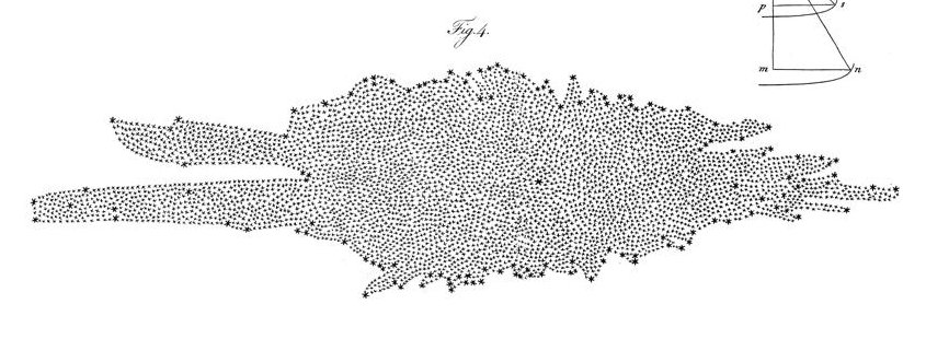
We have not always known what galaxies are. This is because astronomers did not always know their distances, as we have discussed in Chapter 13: The Expansion of the Universe. For a long time, astronomers lacked any techniques that could be used to measure the distances to them. In the early 18th century, it was clear the Milky Way could be resolved by telescopes into individual stars; however, some astronomers debated whether or not other faint objects were within or beyond its reaches. In the late 18th century, William Herschel (1738 - 1822) and his sister Caroline Herschel (1750 - 1848) mapped the distances to stars in multiple directions based on a simple assumption; all stars are of the same intrinsic brightness. Today we know this is a grossly flawed premise. The intrinsic brightness of stars (their luminosity) ranges from a thousand times dimmer than the Sun to a million times brighter than the Sun. Nonetheless, the Herschels made progress on one idea that has been shown to be true: we live within a flattened disk of stars (Figure 14.3).

Figure 14.3: Herschel’s drawing shows a section of the Milky Way from his 1785 paper, “On the Construction of the Heavens.” Credit: Herschel, W. (1785) Philosophical Transactions of the Royal Society of London, 75, 213

It was another 130 years before Jacobus Kapteyn (1851 - 1922) could estimate distances to stars with statistical analysis of stellar parallaxes and proper motions of nearby stars. While the methods used by Kapteyn neglected the effects of intermediate gas and dust blocking light from distant stars, he did succeed in confirming the Sun is not in the center of the Milky Way. He also provided astronomers with the scale and extent of the Galaxy. The Kapteyn Model published in 1922 depicts the Milky Way as a flattened disk approximately 50,000 light-years in diameter and about 10,000 light-years thick. Today we know it to be 100,000 light-years in diameter and about 3,000 light-years thick.

Even with the size of the Galaxy known, there was still disagreement over other objects. In 1781, Charles Messier (1730-1817) had assembled his Messier Catalog of 110 celestial objects, a favorite among amateur sky watchers because of the accessibility of its objects to small telescopes. Initially developed to distinguish permanent objects from transient comets, this catalog contained numerous diffuse objects distinguishable from solitary stars. As the resolving power of telescopes increased, astronomers could identify individual stars making up many of objects, all called nebulae at that time. With this, the distance to Messier objects became hotly debated. Are they objects within the Milky Way or are they something beyond? The only way to settle this argument was to determine accurate celestial distances.

In 1925, Edwin Hubble was the first to show that one of the dim objects in this catalog, Andromeda, was actually a neighboring galaxy. Hubble did this using the Cepheid period-luminosity relationship that had recently been developed by Henrietta Leavitt - see the discussion in Chapter 13.1. We now know that some of the objects in Messier’s catalog are other galaxies (outside our Galaxy), while others are star clusters and nebulae within the Milky Way.

As we have already seen, Hubble’s Law relates the recessional velocity of a galaxy to its distance.

\[v=H_0d \nonumber \]

In this expression, v is the velocity of a galaxy, d is its distance, and H₀ is a constant of proportionality called the Hubble constant. This relationship is a consequence of the expansion of space, and it causes a cosmological redshift. The farther away a galaxy is, the faster its velocity and the greater its redshift. The relationship between velocity and cosmological redshift are given the equation below, as discussed earlier.

\[v=cz \nonumber \]

In this expression, v is the velocity of a galaxy, z is its redshift, and c is the speed of light. This is valid when redshifts are small. Combining these two equations, we get:

\[cz=H_0d \nonumber \]

We can rearrange terms to obtain an expression for distance in terms of redshift:

\[d=\dfrac{cz}{H_0} \nonumber \]

Once we have determined the value of the Hubble constant by using a sample of galaxies (as Hubble did), we can then turn around and use the relationship to determine the distance to any galaxy. We need only measure the redshift of the target galaxy! You will practice this technique in the next activity. This method does not give extremely accurate distance determinations for individual galaxies because there is a lot of scatter in the Hubble relation. Nonetheless, it does give us an idea of the distance to any galaxy from which we are able to obtain a spectrum.

Redshift and Distance

In this activity you will assume a value for the Hubble constant and use that to calculate the distances to galaxies given their redshifts.

Worked Example:

1. A galaxy has a redshift of 0.02. Assume the Hubble constant is 70 km/s/Mpc. What is the distance to this galaxy?

• Given: z = 0.02, H₀ = 70 km/s/Mpc, c = 3e5 km/s
• Find: d
• Concept: d = cz/H₀
• Solution: d = (3e5 km/s) (0.02) / (70 km/s/Mpc) = 85.7 Mpc

Questions:

1.

2.

3.

In the previous activity you learned how to compute a galaxy’s distance from its redshift. To measure a galaxy’s redshift, it is only necessary to take its spectrum. This is a much less labor intensive way to measure the distances to galaxies than other techniques. Redshift surveys have allowed astronomers to map the Universe in three dimensions on a massive scale.

Building a comprehensive map of distant objects requires broad surveys of galaxies near and far all over the sky. Modern surveys like the Sloan Digital Sky Survey (SDSS), the 2 Micron All Sky Survey (2MASS) (Figure 14.4), and the 6dF have measured redshifts for millions of galaxies.

Figure 14.4: Pictures of SDSS (left) and 2MASS (right) telescopes, which carry out galaxy surveys. The SDSS telescope, which maps the sky in optical (visible) light, is located at the Apache Point Observatory in New Mexico. Prof. Connie Rockosi of UC Santa Cruz was part of the team that built the camera for the survey. The 2MASS telescope pictured here is located at Mt. Hopkins in Arizona; there is a second telescope located in Chile. Both of the 2MASS telescopes map the sky in infrared light . Credit: Image courtesy of Sloan Digital Sky Survey; Image courtesy of 2MASS/UMass/IPAC-Caltech/NASA/NSF

The SDSS canvassed more than 25% of the night sky for 8 years from 2000 to 2008. Since 2008, SDSS has continued to do astronomical observations with specific scientific goals that include deeper studies of the Milky Way galaxy, exoplanets, and cosmological measurements. To date (through 2013), SDSS has gathered multi-color images and spectra of over 1.8 million galaxies, and for more than 300,000 quasars. SDSS uses a 120-megapixel camera; it can snap a picture 8 times larger than the full Moon and record spectra for more than 600 objects at a time. This is an enormous amount of data. On a typical day, SDSS could process over 12 terabytes, or 12,000 gigabytes, of data.

Dust and gas in the plane of the Milky Way obscures the views of optical surveys like SDSS. To provide an unprecedented view into this “zone of avoidance,” 2MASS charted the sky in dust-penetrating infrared light. Observations with 2MASS were taken between 1997 and 2001 in Arizona and Chile. Throughout its run, the survey collected nearly 25 terabytes of data. After image processing, the final database of 12 terabytes has been made available to the public.

With these surveys we see that on the largest observable scales, galaxies and clusters are found in thin, filamentary web-like structures forming walls with large bubbles mostly devoid of galaxies (Figure 14.5). Shown on top is one slice of galaxies in the SDSS survey. Earth is at the center of this map, and the distance away from us for these objects is represented here using redshift, z. Shown on the bottom is an all-sky map from 2MASS.

Figure 14.5: (Top) This is a slice through the 3-dimensional map of the distribution of galaxies from the SDSS survey. Earth is at the center and each point represents a galaxy, typically containing about 100 billion stars. Galaxies are colored according to ages of their stars. Red is old and green is young. (Bottom) The 2MASS all-sky catalog. Again, each point is a galaxy. The blue haze is the area obscured by our Galaxy. Both SDSS and 2MASS reveal that the large-scale structure of our Universe resembles a web. Credit: M. Blanton and the Sloan Digital Sky Survey; 2MASS/T.H. Jarrett, J. Carpenter, & R. Hurt

The Sloan Digital Sky Survey

In this video, you will see a rotating view of a three-dimensional plot of the galaxies in SDSS as of 2004. Each dot in the video is a galaxy. They survey is being conducted in large wedges looking out from Earth. As more data are collected the space between the slices will start to fill up.

1.

(A) (B)

Figure 14.A.1: Some ideas for what the large-scale structure might look like. What do you think? Credit: Daniel Smith, South Carolina State University; Zoe Buck

Credit: Sloan Digital Sky Survey

After you have watched the video, answer the following questions:

2.

3.

4.

5.

6.

7.

From SDSS data, we can identify several features. Galaxy filaments are massive string like formations typically 150 - 300 million light-years long. Galaxy nodes sit at the intersection of galaxy filaments. Sheets of galaxy filaments form massive walls which in turn outline the bubble-like voids. The statistics of voids, including their size and distribution, are closely tied to cosmological parameters and the detailed physics of structure formation. Surveys and simulations show that the voids tend to be around 100 million light-years in diameter. Estimates put the total volume of voids at roughly 40% of the total volume of the Universe.

Large Scales of the Universe

Play Activity

In the early part of the 20th century, scientists like Einstein were using the theory of general relativity to describe the behavior of the Universe. Astronomers studying the Universe made a simplifying assumption that is now known as the cosmological principle. It states:

On the largest cosmic scales, the Universe is both homogeneous and isotropic.

Homogeneity means that there is no preferred location in the Universe. That is, no matter where you are in the Universe, if you look at the Universe, it will look the same. Isotropy means that there is no preferred direction in the Universe. That is, from your current location, no matter which direction you look, the Universe will look the same. When we say “the same”, we do not mean identical. Rather, we mean that if we analyze statistical properties that describe how matter is distributed, we will get the same results in any direction and at any location (when we analyze large enough areas). Can we test if this is true?

At first glance, diagrams like Figure 14.5 of the distribution of galaxies in the Universe seem to imply that the Universe is not homogeneous and isotropic. They make it seem that galaxies in one direction are not distributed in the same way as the galaxies in another direction. However, the galaxies in the SDSS slice shown only extend to a redshift of z ~ 0.15 and in the 2MASS map to z ~ 0.1. As we study objects to larger distances, the structure does smooth out and become more homogeneous on larger scales. In Animated Figure 14.6, we see layers of the 2MASS survey at increasing redshift that show greater homogeneity with increasing distance. When statistical analyses are made on luminous galaxies and quasars in the SDSS catalog out to redshifts of ~0.6 and 1.8 respectively, the Universe is found to be homogeneous on scales of 400 – 600 million light-years and greater. Thus, we currently find support for the cosmological principle in the distribution of galaxies in the Universe.

Animated Figure 14.6: This movie shows layers of the 2MASS survey at increasing redshift, or equivalently, increasing distance. On larger scales, the distribution of matter becomes more homogeneous. Credit: Movie courtesy of 2MASS/UMass/IPAC-Caltech/NASA/NSF

GOING FURTHER 14.1: LARGE QUASAR GROUPS

The Formation of the Largest Structures

Galaxies, clusters of galaxies, and super-clusters of galaxies make up the large-scale structures that we observe as part of the cosmic web. But how did these structures form?

The Universe is expanding, consistent with the Big Bang theory: the Universe was much hotter and denser in the past, and it changes as it expands and cools. Structure formation happens in this context. A complete cosmological framework should be able to explain the structures we see, not just the fact that the Universe is expanding, but that it contains galaxies and other structures. Furthermore, the model should naturally connect the early epochs in the history of the Universe to current conditions in a natural way.

Structure formation models therefore must begin when the Universe was a hot, dense plasma that was much more uniform than the lumpy Universe we see today. Initially tiny fluctuations present in the early Universe grew by gravitational attraction into the magnificent large-scale structures that we observe in galaxy surveys. We should see signs of this structure in all phases of the Universe's evolution, for instance, in the Cosmic Background Radiation.

When the Universe was about 500,000 years old, the density of matter in a region of space that would eventually form a galaxy was about 0.5% higher than the density of its surroundings. At that time, denser regions of space expanded more slowly than other regions of space because the pull of gravity was higher in the regions with a higher mass density. As a result, denser regions became even denser compared to surrounding regions. When the Universe was ~15 million years old, dense regions, like the one that eventually formed the Milky Way galaxy, were about 5% denser than surrounding regions. This enhancement continued. By the time the Universe was about a billion years old, typical collections of matter were about a factor of two denser than their surroundings. At the present time, the disk of the Milky Way is about a factor of 1000 denser than its halo, which is in turn about a factor of 1000 denser than the Universe on average.

At first, when the density was nearly uniform everywhere, with only small variations (10^-4 to 10^-5), gravitational collapse proceeded in a straight-forward linear manner. As more matter collected in the denser regions, eventually the fluctuations became equal to the average density and the gravitational collapse became non-linear. The scenarios for how structure could have formed in this gravitational attraction framework are modeled with the aid of computers. One class of models works well for the so-called linear regime, when fluctuations were still small. These models start when the Universe was about 10,000 years old and continue through the formation of the cosmic microwave background at 380,000 years. They are able to generate statistics for the distribution of galaxies on the largest scales, and these can be compared to observations of the real universe. The second class of models, which will be the focus of this chapter, explores the non-linear regime of larger scale structure formation that follows.

The computer simulation in Figure 14.7 illustrates how large-scale structures form over time. They show an enhancement of density as time progresses, a result of gravitational attraction. Computer simulations of the growth of large-scale structure include the laws of physics, such as gravity and thermodynamics, and track the motions and energy of cold dark matter and regular (baryonic) matter. Most of the mass of the Universe is cold dark matter, not baryonic matter, so structure formation is dominated by dark matter; baryonic matter is attracted to and enhances the structures initially created mainly by the clumping of dark matter.

Figure 14.7: Simulation of the growth of large-scale structures. The Universe gets lumpier as time progresses due to gravitational attraction. This simulation ran from a redshift of z = 30, when the age of the Universe was about 100 million years old, to today (z = 0). The size of the box is 140 million light-years wide today. The coordinates are co-moving with the expansion of the Universe so that the same patch of sky is shown in each box, even though the size of the box is much larger at recent times. Credit: Simulations were performed at the National Center for Supercomputer Applications (NCSA) by Andrey Kravtsov (The University of Chicago) and Anatoly Klypin (New Mexico State University). Visualizations by Andrey Kravtsov.

How do the large structures of the cosmic web form if the key driving force is the gravitational pull of dark matter? Since gravity pulls inward in all directions, you might at first guess that large clouds of matter would remain spherical as they collapse. In fact, we find many other shapes on the largest scales. In the next activity, we will consider what happens to the more general shape of an ellipsoid.

Collapse of Clouds of Matter

A roughly spherical cloud of matter can be perturbed such that each of three axes is a slightly different length. The cloud will then be shaped like an under-inflated football that someone squished. The football-shaped object has a long axis (c) that passes through the pointy ends and two additional axes, one through the squashed face (b) and another perpendicular to it (a) as shown in Figure A.14.2.

Figure A.14.2: An ellipsoidal cloud of matter. The shortest axis collapses faster than the rest, forming a disk. The next shortest axis collapses forming a filament. Finally, the third axis can collapse to form a node. Credit: NASA/SSU/Aurore Simonnet

The gravitational force between any two objects with mass is given by Newton's Law of Gravitation.

\[F=\dfrac{GM_1M_2}{r^2} \nonumber \]

In this equation, r is the distance between two objects of mass M₁ and M₂. For illustrative purposes, we will consider four identical clumps of matter: one sitting at the center of Figure A.14.2 and one at the end of each axis, a, b, and c which we will call clumps A, B, and C, respectively.

Questions

1.

2.

3.

From this activity we see that clumps of matter along the shortest axis will accelerate faster toward the center than matter along the largest axis. If we watch a simplified movie of gravitational collapse, this cloud of matter will first collapse from an ellipsoid to a pancake, then a rope, and finally a condensed ball. In this way, matter in the Universe formed into numerous massive sheets (walls), many of which further collapsed into cylinders (filaments), and within these large filaments, or at their intersections, we finally get compact nodes. We can get this great variety of shapes even without considering rotation.

Animated Figure 14.8 is a computer simulation showing the formation of the cosmic web. The simulation begins with a nearly uniform volume of gas at high redshift and runs through the present day. We then fly though the survey, zooming in on structures that might resemble the Local group and Virgo cluster. This simulation, and others like it, include the laws of physics, such as gravity and thermodynamics. They model the evolution of both regular and dark matter. The output of the simulations closely matches the cosmic web pattern observed in galaxy surveys.

Animated Figure 14.8: This simulation by the CLUES Team shows the formation of large-scale structure in the Universe and then zooms in on more local structures. The box size is 275 light-years in co-moving coordinates. This movie shows the evolution of dark matter, though the simulation also includes baryonic matter. Credit: CLUES team and C. Henze, N. McCurdy, J. Primack

Using these models, we can probe various cosmological parameters, or aspects in the models that tell us about the nature of the Universe. Model parameters include the amount and nature of the matter and energy in the Universe and the types and strength of initial fluctuations. For example, each panel in Figure 14.9 shows a different pattern for the distribution of galaxies because each uses a different set of parameters. By comparing simulations of differing parameters with data from galaxy surveys we can determine the best-fit values of the parameters; we can infer that the models with the best fit to the data tell us the properties of our Universe.

Of course, there are often many ways to adjust model parameters to obtain similar fits because different parameters can counteract one another. For this reason, it is not always straightforward to make conclusions based upon a single model, or even several models. Nevertheless, as our models increase in their level of sophistication, and different sets of models by different researchers give us complementary and consistent ways to understand the data, our confidence increases that many aspects of our views of the growth of structure must be correct, at least in general outline.

In the next activity you will run a simple cosmological simulation with only two parameters and find a best-fit match to SDSS data.

Figure 14.5, in order to determine the best fit values of the parameters. Credit: C. P. Ma, University of California, Berkeley

Structure Formation and Cosmological Parameters

In this activity, you are going to match the output of a large-scale structure simulation to data from galaxy surveys in order to determine the value of two cosmological parameters: the density of matter (Ω_m) and the amplitude of fluctuations (σ₈).

• The matter density, here written as Ω_m (Greek letter “Omega”), is the ratio between the matter density to the critical density; Ω_m is a number between 0 and 1.
• The amplitude of fluctuations, here written as σ₈ (Greek letter “sigma”), is a measure of how strong the fluctuations are on scales of 8 Mpc (26 million light-years).

Now go to the simulation website:

Play Activity

Click "Launch Interactive Lab" (on the picture in the middle of the page).

A. The effect of changing parameters.

1.

2.

B. Best fit parameters.

Run the simulation with different values of Ω_m and σ₈ until you find the values that best match the observed image and histogram

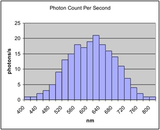
Click “check answers” to see if you are correct.

Enter the best fit values for Ω_m and σ₈ here:

1.

2.