16.3: Inflation

Learning Objectives

• You will know that magnets are never seen as single poles and that and explanation for this led to a theory with cosmological implications.
• You will know that the Universe underwent a period of rapid, exponential expansion at early times.
• You will understand how inflation can explain the observed homogeneity and isotropy of the Universe.
• You will understand how inflation can explain the observed flat geometry of the Universe.
• You will know that inflation is driven by a release of energy from the field of a particle known as the inflaton.
• You will know that inflation makes predictions about structure formation, which can be tested.

What Do You Think: Inflation

The Big Bang theory explains a lot of what we see in the Universe very well. However, it cannot be complete. For example, the Big Bang theory does not explain why the Universe is isotropic and homogeneous on large scales. It also fails to explain why the geometry of the Universe is flat. Clearly there was something early in the history of the Universe that set up these conditions, but the original framework of the expansion model does not say what that was. Surprisingly, it was not from astrophysics that the best explanation for these observational puzzles arose. The explanation of the appearance of the Universe on the largest scales came from an attempt to understand a puzzle from other branches of physics. To understand how this happened, we will take a brief excursion into the physics of electromagnetism.

Magnetic Monopoles: A Puzzle From Particle Physics And Electromagnetism

By now you are familiar with the particle constituents of atoms: protons, neutrons, and electrons. You also know that protons and electrons have electric charge, whereas neutrons do not. In the classical theory of electricity, an electric field can be created by charged particles, so both the electron and the proton create an electric field in the space around them (Figure 16.18). On the other hand, the neutron, lacking an electric charge, does not create an electric field.

Figure 16.18: The electric field configuration for single negative electric charges like electrons. The electric field lines are directed radially inward for a negative charge (as indicated by the arrows in the figure). If the charge is positive, the field lines are directed radially outward. The arrows indicate the direction of the force that the field would exert on a positive charge placed in a given position. For a negative charge placed there, the force would be in the opposite direction, so opposite the direction of the electric field. Credit: Aurore Simonnet

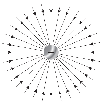
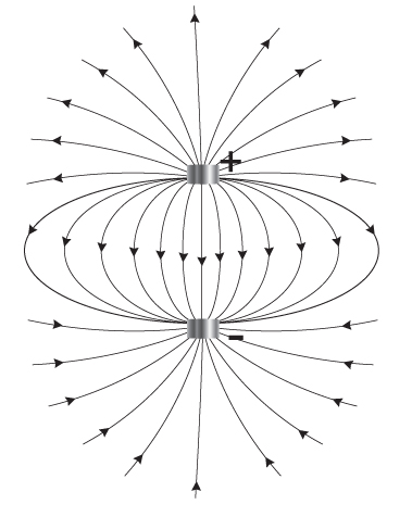
For electric fields, the simplest type of field, as in Figure 16.18, is formed at a charged point-particle and flows radially inward or outward from that charge. Such a configuration is called a monopole field because only a single positive or negative charge (a single pole) is required to produce it. If two charges are close together, their fields interact to produce a dipole field, as shown in Figure 16.19. In this case there are two poles rather than one.

Figure 16.19: Electric dipole fields are created when two charges are in close proximity. Here we show the field for a dipole composed of opposite charges. As above, the arrows indicate the direction of the force exerted by the field on a positive charge placed at a given position. Credit: Aurore Simonnet

On the other hand, a magnetic field is formed in a very different way. Magnetic fields are created when an electrically charged particle moves through space. For example, magnetic fields form around wires carrying electrical currents. Currents are just streams of charged particles (generally electrons) moving in the wire. However, there are no individual “magnetic charges” as there are electric charges, so we do not see magnetic fields that look like the field shown in Figure 16.18. There is no known fundamental reason why there cannot be magnetic charges. In fact, some basic theories of particle physics suggest that such particles should exist. Still, none has ever been seen.

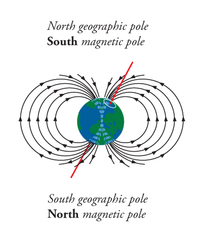
The simplest field configuration for a magnetic field always has two poles, called north and south, in reference to Earth’s magnetic field, shown in Figure 16.20. Since there don’t seem to be any individual magnetic charges, or if you like, no magnetic monopoles, it is not possible to create a magnetic monopole field.

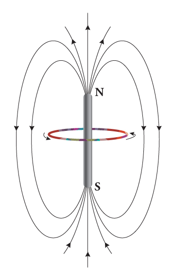
The simplest magnetic field is a dipole field, shown in Figure 16.21. Note that the geometry of this field is the same as the geometry of the electric dipole shown in Figure 16.19. Only the geometry is the same here, the fields are not. One is an electric field, the other is a magnetic field. These are quite different, and they are formed in different ways, but related, ways. Unlike the electric field, the magnetic field is never created by isolated magnetic poles, and this lack of magnetic monopoles has had a profound influence on our understanding of the Universe.

Figure 16.20: The magnetic field of Earth has a characteristic shape called a magnetic dipole. The field has two poles, one near the north geographic pole and one near the south - though the magnetic poles wander around somewhat on the surface. This field configuration is the simplest kind of magnetic field observed. Credit: Aurore Simonnet

Figure 16.21: A magnetic dipole. Magnetic fields cannot have monopole configurations because they are formed by moving electric charges; there are no individual magnetic charges analogous to electric charges. Breaking a magnet in half does not result in isolated north and south poles. It creates two smaller magnets, each having its own north-south pole pair. Credit: Aurore Simonnet

Physicists long puzzled over why there are no magnetic monopoles. From pure symmetry grounds it seems that there should be. The equations describing the electric and magnetic fields are precisely symmetrical, or would be if there were magnetic monopoles analogous to electric charges. Such a particle would appear to be an isolated north or south pole. But in actual magnets the north and south poles always come in pairs. It is as if electrons and protons always came in pairs that could not be broken apart, so we only could see the electric dipole field of the pair, never the two separate charges.

In the 1970s and 1980s GUT theories were predicting that huge numbers of stable magnetic monopoles should have been made in the Big Bang, yet none had ever been detected. Such a large number magnetic monopoles were predicted in these theories that small loops of wire with a steady current would have been measurably disturbed by the close passage of a monopole about once every day. A couple of claims for detection were made, but none were convincing. Where, then, were all of the expected monopoles? This was a question that particle physicists set out to answer.

Of course, it was always possible the theories predicting monopoles were simply wrong, but other possibilities were also explored. It is these explorations that to the idea of this section: Inflation.

The Inflationary Paradigm

An interesting solution to the so-called monopole problem was devised independently by several theoretical physicists in the late 1970s and early 1980s. All of these solutions employed the concept of vacuum energy, the energy of “empty” space. Such vacuum energy has a negative pressure associated with it, something like the tension in a taut cord. In general relativity, this produces a repulsive effect. This repulsive force is the essence of the solution to the monopole problem. As it happens, it also solves many puzzling aspects of Big Bang cosmology as well.

Imagine a region of space that is empty of all matter. The region, though lacking matter, will still contain various fields. According to quantum physics, the presence of these fields will cause the region to have an energy associated with it. The energy results from a sea of virtual particles that constantly pop in and out of existence. To create additional empty space, it is necessary to furnish the energy in the vacuum it contains. This has the effect of producing a resistance to the creation of more empty space. This very resistance produces a negative pressure. Thus any small volume of space will repel adjacent volumes, paradoxically causing the creation of additional space. The energy of the newly created space is the same as that of the original, so the process of expansion is ongoing. In fact, as more space is created, it tends to cause the space to expand ever faster.

But how can the energy of this expansion arise? It can come from the decay of one of the fields in space. Just as an excited atom can decay when an electron drops to a lower energy state (releasing energy in the process) an excited field can also decay. If it does, then something quite extraordinary can happen. As the field decays, the energy released can create new particles. It can also cause space to expand, and by an immense factor.

It is now thought by many cosmologists that just such an expansion took place in the earliest moments after the Big Bang, and this brief period of rapid expansion is now generally referred to as Inflation. A young theoretical physicist named Alan Guth (b. 1947, Figure 16.22) stumbled upon this discovered around 1979 while he was trying to understand something else entirely: why no magnetic monopoles ever showed up in physics experiments. Early breakthroughs also came independently by Alexei Starobinsky (b. 1948) and Andrei Linde (b. 1948) in the Soviet Union. However, it was Guth who first saw the importance of the idea for cosmology.

Figure 16.22: A recent picture of Alan Guth. Credit: Betsy Devine / CC-BY-SA-3.0

Guth’s discovery suggested a reason for the lack of monopoles: even if the Universe had been filled with monopoles at its birth, a phase of rapid expansion as envisioned above would so dilute them as to make it seem as though none existed at all. In this brief period of Inflation, the Universe expanded by at least a factor of 10²⁰, and possibly by a much larger factor (Figure 16.23). That means that two particles originally a micron apart at the beginning of the Inflationary epoch would end up 10²⁰ times farther away, or at least 10¹⁴ m apart at the end of Inflation. This is a size several times larger than the solar system. The rapid expansion would extend across the entire part of the Universe in which the inflationary field was decaying, and any monopoles would be swept across the horizon as space rapidly expanded.

Figure 16.23: During a brief period of inflation, the size of the Universe expanded exponentially. Credit: NASA/SSU/Aurore Simonnet

Monopoles might or might not exist, so having a mechanism that would make them extremely rare is interesting, but not really compelling. However, Guth soon realized that Inflation would also have striking effects on appearance of the Universe as a whole, addressing key issues that the basic Big Bang theory does not.

Inflation Solves the Horizon Problem

So far we have seen that the Universe on the whole is homogeneous and isotropic. If we look in one direction in space we can see objects that are now tens of billions of light years away. When we look in the opposite direction, we see other objects similarly distant. Both regions look strikingly similar. Why should that be? They are so far from each other that nothing (not even light) can have passed between them to coordinate conditions. They are beyond each other’s cosmic horizons (the distance that light has traveled since the Universe began). This mystery, on which a simple Big Bang theory is silent, is called the horizon problem.

The horizon problem is most striking in the cosmic microwave background. It has essentially the same temperature to a tiny fraction of a kelvin all around the sky. How did this condition come to be if these parts of the Universe were never able to exchange information or energy? Inflation provides a way.

Imagine a handful of patches of space close together only an instant after the expansion of the Universe began, but before the onset of Inflation. The regions will experience two effects. The expansion will stretch them away from each other, but as time passes they will also be able to see things farther away as light has more time over which to travel. They might all start with unique properties. Do they have the opportunity to share those properties or are they stretched away from each other too quickly?

In the standard Big Bang model they are always stretched away too quickly. The solutions of the Friedmann equation for radiation and matter dominated Universes all have a stretching rate that approaches infinity as we approach t = 0. Even though the horizon distance for each patch of space will grow as light speed times the elapsed time, that is no match for the stretching rate, and the patches are never able to exchange energy.

If, however, the Universe had an episode of Inflationary growth early in its history, the stretching could have started slowly before accelerating to a high rate. That would provide more time for sharing. In addition, the tiny regions that were able to share energy were inflated to regions much larger than we can currently observe. So even if the entire Universe has diverse properties on very large scales, on scales the size of our visible Universe it is homogeneous. Thus inflation solves the horizon problem, creating the homogeneous and isotropic conditions we observe.

Inflation Solves the Flatness Problem

In a Universe described by general relativity, space can have an overall, or global, curvature. It can be flat (zero curvature) and follow the familiar Euclidian rules of geometry (parallel lines never meet, triangles have three internal angles that always sum to 180 degrees, the circumference of a circle is \(\pi\) times the diameter, etc.), but it can also be curved and follow other rules. There is nothing in the basic Big Bang theory that requires the curvature of the Universe on the largest scales to have any particular value. But observations of the CMB have allowed us to measure the curvature to a precision of less than one percent, and they show it to be flat.

Why should the curvature be close to that special value? There are far more ways to create a Universe with high curvature than one that is precisely flat. Why should the Universe appear to be "fine tuned" in this way? Perhaps there is a good reason for it, but there is nothing in the standard Big Bang theory that says it should be flat. It seems a strange and unsettling coincidence. This is called the flatness problem.

Einstein’s equations of general relativity tie the curvature of the Universe as a whole to its average matter and energy density. A flat geometry results only if the Universe has the critical density, with a precise balance between runaway expansion and runaway collapse. This seems extremely unlikely. But the Universe does seem to be in this special state. For the overall density to be equal or close to this special density today means it must have been even closer at earlier and earlier times. If the density is even a little bit off from the critical value at some time, at any latter time it will be further off. For more on why this is so puzzling, see Going Further 16.3: Why the Flatness Problem Is a Problem.

Inflation provides a way out of this puzzling situation. If the Universe expanded by a huge amount early in its history, then any curvature would be greatly diminished on the scales we can measure. As an analogy, consider Earth’s surface. Globally it has a geometry resembling a sphere. However, standing on the ground you do not notice its curvature. Standing on a tall building in Chicago and looking around you, Earth’s surface still seems to be flat. It will even appear flat if you stand on a high mountain above the California coast and look out to sea. Even if you look out the window of a jet aircraft cruising aloft, Earth appears flat. None of these perspectives lets you discern Earth’s global curvature. The size of the planet is so vast that its global curvature is completely hidden on such small scales.

A similar situation applies to the Universe after Inflation. Even though the Universe might have some global curvature, Inflation expanded it so much that we can currently see only a tiny fraction of it. On these relatively tiny scales, and even on larger ones, the Universe appears flat. This is notwithstanding its global geometry. That is how Inflation solves the flatness problem: it inflates it away, as is depicted in Figure 16.24.

Figure 16.24: As the scale factor of the Universe grows exponentially during the time of inflation, any curvature becomes less significant, to the point of looking flat. Credit: NASA/SSU/ Aurore Simonnet

Going Further 16.3 Why the Flatness Problem Is a Problem

The coincidence of a flat Universe, or in other words, one with a density equal to the critical density, is quite special. Since there is no particular reason that the Universe should be close to the critical density, it is strange that it does lie so close.

If the density of the Universe is equal to the critical density, the expansion rate exactly equals the rate needed to make the Universe flat, so the Universe would expand forever but at a velocity always slowing towards zero. Understanding why this is the case is difficult without mathematics, so let’s try a simplified illustration.

We will use an analogy to the Newtonian notion of the escape speed from a planet. For illustrative purposes we can replace the expanding Universe with a single object leaving a planet at escape velocity, depicted in Figure B.16.3. The physics will be qualitatively the same, but the mathematical treatment is much simpler in the Newtonian case. If we reduced that object’s velocity by 1% it would no longer escape but would turn around and fall back. For example, if we launch a rock off of Earth’s surface at 99% of the escape speed, the rock would get almost all the way to the Moon before it stopped and fell back to Earth.

If we fancifully imagine that the planet at earlier times was compressed to smaller radii (the way the size of the Universe is smaller at earlier times), then we will find a striking effect. Launching our rock with the same 99% of the escape velocity for a compressed planet will hardly raise it off the surface at all before it falls back. For example, to get to the Moon’s orbit with a compressed Earth, we would have to launch the projectile with a higher velocity, greater than 99% though still slightly less than the escape velocity. The following activities show why this is so.

In this Newtonian example, the velocity of the object gets closer and closer to the escape speed as a planet gets smaller, analogous to the density of the Universe getting closer and closer to the critical density as the size of the Universe shrinks at earlier times.

Figure B.16.3: Object Launched from a Planet Surface. If an object with mass m is launched at some velocity v from the surface of a planet with mass M, how far up does it go before it stops and falls back down? Credit: NASA/SSU/Aurore Simonnet

If an object of mass \(m\) is thrown upward with speed v from the surface of a planet it will have a total energy (\(E_{tot}\)), which is a combination of kinetic and potential energy, given by the equation below.

\[ E_{tot}=\frac{1}{2}mv^2 - \frac{GMm}{R} \nonumber \]

Here \(M\) is the mass of the planet and \(R\) is its radius. If we assume that the velocity is less than the escape velocity and the projectile eventually rises to the point \(r\), then the total energy can also be written as follows.

\[ E_{tot}= - \frac{GMm}{r} \nonumber \]

Setting these two expressions equal to each other we can relate the distance traveled to the size of the planet.

\[ \frac{GMm}{r}= \frac{1}{2} mv^2- \frac{GMm}{R} \nonumber \]

The escape velocity is found by setting the total energy to zero. (In that case the object will eventually have no kinetic energy, and its potential energy will be zero since \(r\) will become infinite.) But we are not looking for the escape speed here, we wish to know how high the object travels before it stops and falls back.

We can cancel the common factor of m from each term, and then solve for \(r\).

\[ \frac{GM}{r}= \frac{1}{2} v^2- \frac{GM}{R} \nonumber \]

Rearranging we get the following relation.

\[ r= \frac{-GM}{\frac{1}{2}v^2-\frac{GM}{R}} \nonumber \]

This expression can be greatly simplified by factoring out the \(GM / R\) from the denominator.

\[ r= \frac{-GM}{\frac{GM}{R} \left(\frac{Rv^2}{2GM} - 1\right)} \nonumber \]

Now we can cancel the common term of GM from the numerator and denominator and raise the factor of \(1 / R\) from the denominator into the numerator. In addition, we see that there is a factor of the escape velocity in the denominator: v²_esc = 2GM / R. Thus we can simplify as follows:

\[ r= \frac{-R}{\left (\frac{v}{v_{esc}}\right )^2-1} \nonumber \]

Now we can tidy up a bit by canceling a factor of -1 from the numerator and denominator of the right-hand side, and we can divide through by R to get a final expression for how high an object rises given a planet’s size and the object’s velocity.

\[ \frac{r}{R}= \frac{1}{1- \left (\frac{v}{v_{esc}}\right )^2} \nonumber \]

We can use this expression to determine how high an object will rise if launched from Earth, as in the following worked examples.

1. How far will an object rise off the surface of a planet (relative to the planet’s radius) if it’s launched at 90% of the escape velocity?

• Given: v = 0.90v_esc
• Find: r/R
• Concept: r/R = 1/[1 - (v/v_esc)²]
• Solution: r/R = 1/[1 – (0.90)²] = 5.26

This means it will rise to 5.26 times the planet’s radius.

2. How far will an object rise off the surface of a planet (relative to the planet’s radius) if it’s launched at 99% of the escape velocity?

• Given: v = 0.99v_esc
• Find: r/R
• Concept: r/R = 1/[1 - (v/v_esc)²]
• Solution: r/R = 1/[1 – (0.99)²] = 50

This means it will rise to 50 times planet’s radius.

So the object will rise to about fifty times the radius of the object from which it is launched.

3. How far is this for Earth, which has a radius of 6400 km?

• Given: R = 6400 km, r/R = 50
• Find: r
• Concept: r = (r/R)(R)
• Solution: r = (6400 km)(50) = 320,000 km

This is nearly the distance to the moon.

We can also plot the distance reached (r/R) versus launch velocity (v/v_esc). To create the graph, we can calculate r/R for several values of v/v_esc, as in Table B.16.1.

Table B.16.1. Velocity and peak height of an object launched from a planet.

v/vesc	r/R
0.0	1.0
0.2	1.04
0.4	1.19
0.6	1.56
0.8	2.78
0.9	5.26
0.95	10.26

From this table, we use the Graphing Tool to graph r/R vs. v/v_esc in Figure B.16.4.

Figure B.16.4 height and escape speed

Figure: The ratio of the height attained to the radius of the planet as a function of velocity in terms of escape speed. Credit: NASA/SSU

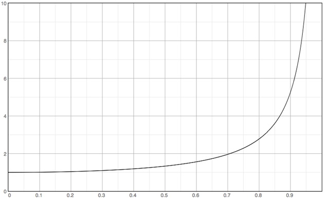
From this graph, we can answer the several questions. You will see that the ratio of launch velocity to escape velocity becomes much more sensitive to deviations from 1.0 as an object shrinks. This is analogous to the expansion of the Universe: the Universe must be very exquisitely balanced near its critical density in order for it to be so close to that density today.

1. Why is the height attained equal to 1 when the launch velocity is zero?

Since the projectile begins at r = R, if it has zero initial velocity it never leaves the surface, so r/R = 1 at its highest point.

2. Explain why the height seems to rise without bound as the launch velocity (in terms of escape velocity) approaches 1.

When v = v_esc the projectile is able to escape to infinity, thus as the launch speed approaches that value the height attained approaches infinity.

3. How does the height reached by a projectile depend on the speed at which it is launched?

As the speed becomes a larger fraction of escape speed the height attained increases, regardless of the size of the planet. The answer does not depend on the size of the planet because both axes on the graph are in terms of the planet’s size. The escape speed includes all of the relevant information on the planet’s mass and radius, and the height attained is in terms of the planet radius, so any dependence on planetary parameters are hidden by this method of plotting.

4. As the planet gets smaller, what must happen to the launch velocity in order to cause the physical height reached by the projectile to remain constant?

If the projectile is to reach a constant value of r as the size of the planet (R) decreases, then its velocity as a fraction of escape speed must increase. Thus the absolute launch speed must also increase.

5. In this exercise, escape velocity is analogous to the critical density of the Universe. How does this exercise demonstrate that, if the density of the Universe today is close to the critical density, it must have been even closer to critical density in the past?

The escape speed of a planet of given mass will increase as the planet is made smaller. That means that if an object is near escape speed on a large planet, it must be even nearer escape speed on a smaller planet of the same mass in order to reach a similar height. The ratio v/v_esc must approach 1 as the planet gets smaller in a way similar to the way that ρ/ρ_crit must approach 1 as we look further into the past when the scale factor of the Universe was smaller than it is today.

Possible Mechanisms for Inflation

The basic starting point for Inflation is the Friedmann equation of general relativity. It predicts that the expansion of a volume of space should slow due to the braking effect of the mass–energy present. However, unlike Newtonian gravity, it also permits a term due to the energy inherent in the vacuum fields of “empty” space. These have an opposite, accelerating effect—a topic we will look at in more depth later.

According to Inflationary theory, most of the energy in the Universe was initially concentrated in an energy field called the inflaton field. Fields are associated with many elementary particles, and usually the energy in these fields is zero. Inflation posits that the field of one particle—the inflaton—got stuck on a non-zero quasi-stable value during one of the force-separating transitions. The inflaton field permeated space and had a large amount of energy stored in the form of vacuum energy. In this case, the vacuum was not a true vacuum, but corresponded to an excited state of the field, called a false vacuum.

When the field began to decay, it released its energy, and since the vacuum energy was tied to space itself, as space expanded, the inflaton field caused the Universe to expand more and more rapidly. As more space was created by the expansion, the total vacuum energy also grew, making the expansion accelerate, and so on exponentially. The size of the Universe doubled over and over in very short periods. We do not know exactly how many doublings there might have been, though the minimum must have been enough to flatten and smooth the Universe on the largest visible scales. During the inflationary stage, the Universe expanded by at least a factor of 10²⁰ or perhaps as much as 10^100000000000 (1 followed by a quadrillion zeros).

The Universe did not remain in such an unstable state for long. Eventually the field decayed to its ground state, a true vacuum. Its energy was converted into other forms, such as particles, and the exponential expansion ceased in favor of a more steady expansion. The energy of the inflaton field may have decayed in what is known as a "slow roll," in which it stayed at a high value for a comparatively long time (though 10^-35 seconds seems fast to most of us!) as if rolling down a hill through honey. Once it was part way down the hill however, the decay accelerated. When the value reached zero, inflation ended. The energy of the field went into repopulating space with energetic particles in a process called reheating. After reheating, the Universe looked almost the same as predicted by non-inflationary models—except all the troubling coincidences (such as the horizon and flatness problems) now make sense and the Universe is much bigger! The possible evolution of the energy of the inflaton field is shown in Figure 16.25.

Figure 16.25: The inflation field started out stuck in a high-energy state called a false vacuum. This state required a long time (by these standards) to decay. While the decay of the field happened slowly, the Universe inflated. When the evolution of the field quickened and its energy dropped rapidly, reheating occurred until the energy of the field hit a true vacuum at zero, ending inflation and creating the mass/energy we see today. Credit: NASA/SSU/Aurore Simonnet

There are many possible theories varying the details of Inflation. In some, the field comes into play at the GUT scale. In others, its effects appear at higher energy scales. Inflation may have begun as early as 10^-43 seconds after the beginning of the Universe, lasting about 10^-35 seconds, or begun as late as 10^-35 seconds, lasting about 10^-32 seconds. Whenever the inflationary epoch was, the exponential expansion it caused gave us the flat, homogeneous, and isotropic Universe we now inhabit.

Additional Observational Tests

As always in science, we insist that ideas like Inflation, which explain so many features of the Universe, must make testable predictions. Inflation makes many such predictions, and we now have the ability to test some of them.

The basic Big Bang theory cannot explain either why the Universe is so homogeneous on billion light-year scales, or why we see any structure at all in the Universe. Why are there galaxies and clusters of galaxies? Why is the CMB slightly lumpy? In the basic Big Bang theory there is no reason for the expansion to be other than perfectly smooth. But a smooth expansion would not have the lumpiness to produce galaxies from gravitational collapse. There must be some mechanism for providing the “seeds” of these structures early in the history of the Universe, so that they can then grow via gravity.

Inflation suggests an answer to this problem too, by providing seeds of inhomogeneity of just the right size. These seeds stem from the inevitable fluctuations on the quantum scale. Inflation would have magnified and frozen-in whatever random set of fluctuations were happening on quantum scales at the moment the rapid expansion commenced. The fluctuations then provided the seeds for the structures we now see on large scales.

Inflationary models also make predictions about the patterns of structures in the Universe, and we can test some of these already. Inflation can provide theoretical seeds of structure that produce models that match the observations of the power spectrum of the CMB to high precision. Furthermore, most inflationary models use fundamentally random seeds to produce structure and the results of these models agree with the structures observed.

The clearest signal of inflation would be a specific signature pattern that would result from the interaction of light with gravitational waves. Inflation is such a dramatic event that it shakes the fabric of space. Gravitational waves created by this shaking would affect the CMB light as it travels through space, imposing a pattern on its polarization.

We have seen that electromagnetic waves have an electric field and a magnetic field perpendicular to each other and to the light’s direction of travel. Most light sources emit light with the electric and magnetic fields oriented randomly, but there are many processes that can favor particular orientations, producing light that is polarized. The effect on light by the gravitational waves generated by inflation should produce a specific pattern of polarization. This effect was tentatively reported by the BICEP team in March 2014. However, upon further analysis with higher quality data from the Planck satellite, the polarization results did not hold up. It is still possible that CMB polarization of the kind predicted by Inflation will be found in the future, but so far (as of 2021 summer), the search for this signal continues.