
9.8: Orbital Elements and Velocity Vector


- Last updated
- Nov 1, 2022
- Save as PDF

( \newcommand{\kernel}{\mathrm{null}\,}\)
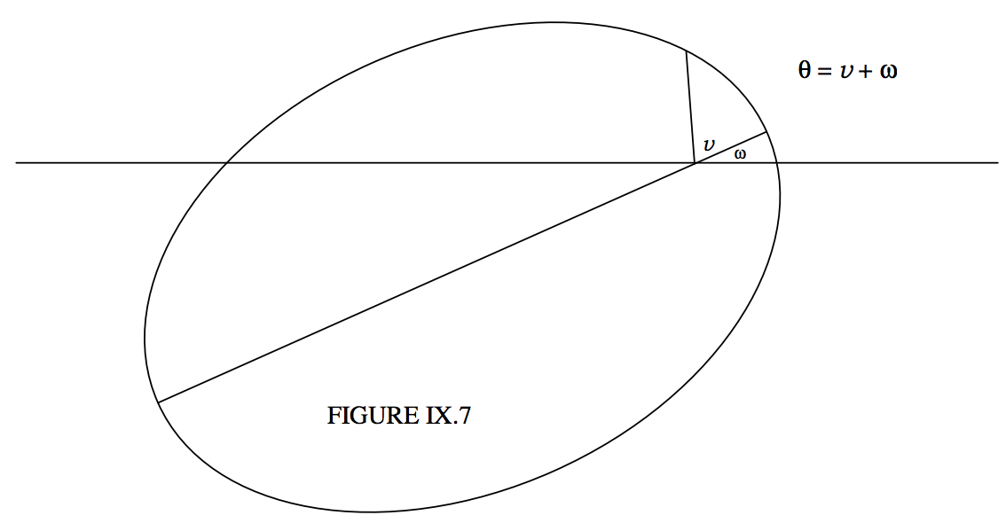
In two dimensions, an orbit can be completely specified by four orbital elements. Three of them give the size, shape and orientation of the orbit. They are, respectively, a, e and ω. We are familiar with the semi major axis a and the eccentricity e. The angle ω, the argument of perihelion, was illustrated in figure II.19, which is reproduced here as figure IX.7. It is the angle that the major axis makes with the initial line of the polar coordinates. Figure II.19 reminds us of the relation between the argument of perihelion ω, the argument of latitude θ and the true anomaly v. We remind ourselves here of the Equation to a conic section
r=l1+ecosv=l1+ecos(θ−ω),
where the semi latus rectum l is a(1−e2) for an ellipse, and a(e2−1) for a hyperbola. For a hyperbola, the parameter a is usually called the semi transverse axis. For a parabola, the size is generally described by the perihelion distance q, and l=2q.
The fourth element is needed to give information about where the planet is in its orbit at a particular time. Usually this is T, the time of perihelion passage. In the case of a circular orbit this cannot be used. One could instead give the time when θ=0, or the value of θ at some specified time.
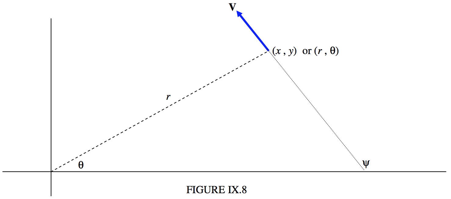
Refer now to figure IX.8.
We’ll suppose that at some time t we know the coordinates (x, y) or (r, θ) of the planet, and also the velocity – that is to say the speed and direction, or the x- and y- or the radial and transverse components of the velocity. That is, we know four quantities. The subsequent path of the planet is then determined. In other words, given the four quantities (two components of the position vector and two components of the velocity vector), we should be able to determine the four elements a, e, ω and T. Let us try.
The semi major axis is easy. It’s determined from Equation 9.5.31:
V2=GM(2r−1a).
If distances are expressed in AU and if the speed is expressed in units of 29.7846917 km s−1, GM=1, so that the semi major axis in AU is given by
a=r2−rV2.
In other words, if we know the speed and the heliocentric distance, the semi major axis is known. If a turns out to be infinite - in other words, if V2=2/r - the orbit is a parabola; and if a is negative, it is a hyperbola. For an ellipse, of course, the period in sidereal years is given by P2=a3.
From the geometry of figure IX.8, the transverse component of V is Vsin(ψ−θ), which is known, the magnitude and direction of V being presumed known. Therefore the angular momentum per unit mass is r times this, and, for an elliptic orbit, this is related to a and e by Equation 9.5.27a:
h=√GMa(1−e2).
rVsin(ψ−θ)=√GMa(1−e2).
Again, if distances are expressed in AU and V in units of 29.7846917 km s−1, GM=1, and so
rVsin(ψ−θ)=√a(1−e2).
Thus e is determined.
The Equation to an ellipse is
r=a(1−e2)1+ecos(θ−ω),
so, provided the usual care is take in choosing the quadrant, ω is now known.
From there we proceed:
v=θ−ω,cosE=e+cosv1+ecosv,M=E−esinE=2πP(t−T),
and T is found. The procedure for a parabola or a hyperbola is similar.
At time t=0, a comet is at x=+3.0, y=+6.0 AU and it has a velocity with components ˙x=−0.2, ˙y=+0.4 times 29.7846917 km s−1. Find the orbital elements a, e, ω and T. (In case you are wondering, a particle of negligible mass moving around the Sun in an unperturbed circular orbit of radius one astronomical unit, moves with a speed of 29.7846917 km s−1. This follows from the definition of the astronomical unit of length.)
Solution
Note in what follows that, although I am quoting numbers to only a few significant figures, the calculation at all times carries all ten figures that my hand calculator allows. You will not get exactly the same results unless you do likewise. Do not prematurely round off. I am using astronomical units of distance, sidereal years for time and speed in units of 29.8 km s−1.
r=6.708, θ=63∘26′, V=0.4472, ψ=116∘34′
Be sure to get the quadrants right!
a=10.19 AU_P=32.5e=0.6593_cos(θ−ω)=−0.21439
And now we are faced with a dilemma. θ−ω=102∘ 23′ or 257∘ 37′. Which is it? This is a typical “quadrant problem”, and it cannot be ignored. The two possible solutions give ω=321∘ 03′ or 165∘ 49′, and we have to decide which is correct.
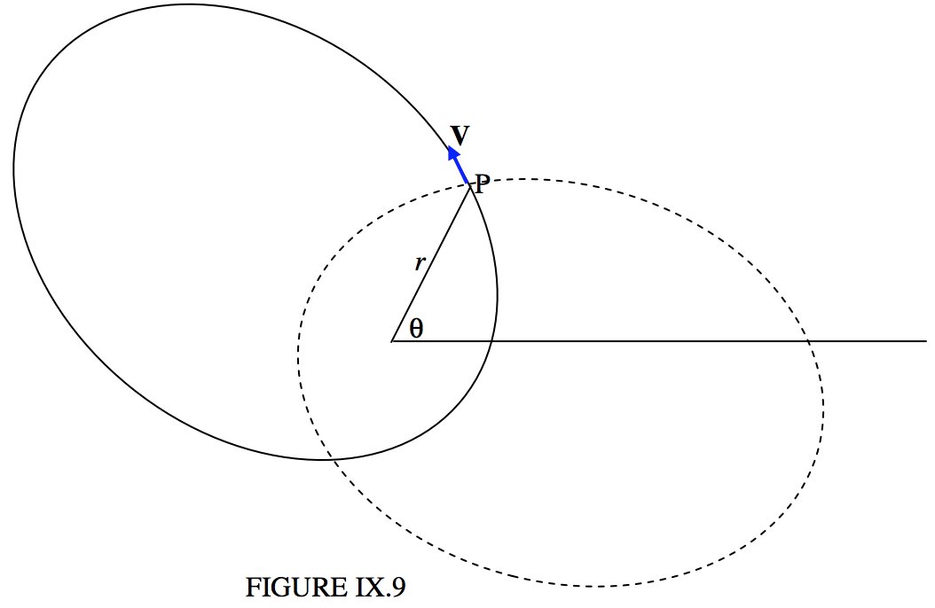
The two solutions are drawn in Figure IX.9. The continuous curve is the ellipse for ω=321∘ 03′ and the dashed curve is the curve for ω=165∘ 49′. I have also drawn in the velocity vector at (r, θ), and it is clear from the drawing that the continuous curve with ω=321∘ 03′ is the correct ellipse. We now have
ω=321∘ 03′_
Is there a way of deducing this from the Equations rather than going to the trouble of drawing the ellipses? I offer the following. I am going to find the slope (gradient) of each ellipse at the point P. The correct ellipse is the one for which ψ=116∘ 34′, i.e. dy/dx=−2. The Equation to the ellipse is
r=11+ecos(θ−ω)=a(1−e2)1+ecos(θ−ω),
from which drdθ=lesin(θ−ω)[(1+ecos(θ−ω)]2.
The expression for dxdy(=tanψ) in polar coordinates is
dxdy=tanθdrdθ+rdrdθ−rtanθ,
and of course r=√x2+y2.
From these, I obtain, in our numerical example,
for ω=165∘ 49′, ψ=190∘, and for ω=321∘ 03′, ψ=165∘49′,
so clearly the latter is correct.
From this point we go:
v=102∘ 23′,cosE=0.51817,
and again we are presented with a dilemma, for this gives E=58∘ 47′ or 301∘ 13′, and we have to decide which one is correct. From the geometrical meaning of v and E, we can understand that they are equal when each of them is either 0∘ or 180∘. Since v<180∘, E must also be less than 180∘, so the correct choice is E=58∘ 47′=1.0261 rad. From there, we have
M=26∘ 29′=0.46218 rad,T=−2.392sidreal years,_
and the elements are now completely determined.
Write a computer program, in the language of your choice, in which the input data are x, y, ˙x, ˙y, and the output is a, e, ω and T. You will probably want to keep it simple at first, and deal only with ellipses. Therefore, if the program calculates that a is not positive, exit the program then. I’m not sure how you will solve the quadrant problems. That will be up to your ingenuity. Don’t forget that many languages have an ARCTAN2 function. Later, you will want to expand the program and deal with any set of x, y, ˙x, ˙y, with a resulting orbit that may be any of the conic sections. Particularly annoying cases may be those in which the planet is heading straight for the Sun, with no transverse component of velocity, so that it is moving in a straight line, or a circular orbit, in which case T is undefined.
Notice that the problem we have dealt with in this section is the opposite of the problem we dealt with in Sections 9.6, 9.7 and 9.8. In the latter, we were given the elements, and we calculated the position of the planet as a function of time. That is, we calculated an ephemeris. In the present section, we are given the position and velocity at some time and are asked to calculate the elements. Both problems are of comparable difficulty. Perhaps the latter is slightly easier than the former, since we don’t have to solve Kepler’s Equation. This might give the impression that calculating the orbital elements of a planet is of comparable difficulty to, or even slightly easier than, calculating an ephemeris from the elements. This is, in practice, very far from the case, and in fact calculating the elements from the observations is very much more difficult than generating an ephemeris. In this section, we have calculated the elements, given the position and velocity vectors. In real life, when a new planet swims into our ken, we have no idea of the distance or of the speed or the direction of motion. All we have is a set of positions against the starry background, and the most difficult part of the problem of determining the elements is to determine the distance.
The next chapter will deal with generating an ephemeris (right ascension and declination as a function of time) from the orbital elements in the real three-dimensional situation. Calculating the elements from the observations will come much later.