11.3.4: Aberration of Light

By “aberration” I am not referring to optical aberrations produced by lenses and mirrors, such as coma and astigmatism and similar optical aberrations, but rather to the aberration of light resulting from the vector difference between the velocity of light and the velocity of Earth. (In these notes, the word “velocity” is used to mean “velocity” and the word “speed” is used to mean “speed”. The word “velocity” is not to be used merely as a longer and more impressive word for “speed”.)

The effect of aberration is to displace a star towards the Apex of the Earth’s Way, which is the point on the celestial sphere towards which Earth is moving. The apex is where the ecliptic intersects the observer’s meridian at 6 hours local apparent solar time. The amount of the aberrational displacement varies with position on the sky, being greatest for stars $90^\circ$ from the apex. It is then of magnitude $v/c$, where $v$ and $c$ are the speeds of Earth and light respectively. This amounts to 20.5 arcseconds. (You didn’t know that the speed of Earth could be expressed in arcseconds, did you?) But what matters in astrometry is the differential aberration between one edge of the detector (photographic film or $\text{CCD}$) and the other. Evidently this is going to be a much smaller effect than differential refraction.

Let us examine the effect of aberration in figures $\text{XI.6a}$ and $\text{b}$.

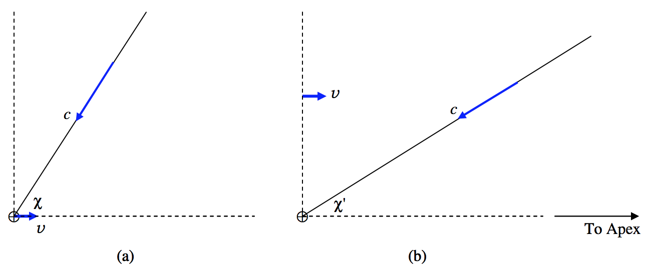
$\text{FIGURE XI.6}$

Part (a) of the figure shows a stationary reference frame. By “stationary” I mean a frame in which Earth, $\oplus$, is moving towards the apex at speed $v = 29.8 \ \text{km s}^{−1}$. Light from a star is approaching Earth at speed $c$ from a direction that makes an angle $χ$, which I shall call the true apical distance, with the direction to the apex.

Part (b) shows the same situation referred to a frame in which Earth is stationary; that is the frame (b) is moving towards the apex with speed $v$ relative to the frame (a). Referred to this frame, the speed of light is $c$, and it is coming from a direction $χ^\prime$, which I shall call the apparent apical distance.

I refer to the difference $ε = χ − χ^\prime$ as the aberrational displacement.

For brevity I shall refer to the direction to the apex as the “$x$-direction” and the upwards direction in the figures as the “$y$-direction”.

Referred to frame (a), the $x$-component of the velocity of light is $− c \cos χ$, and referred to frame (b), the $x$-component of the velocity of light is $− c \cos χ^\prime$. These are related by the Lorentz transformation between velocity components:

$$c \cos χ^\prime = \frac{c \cos χ + v}{1 + (v/c) \cos χ}. \label{11.3.8} \tag{11.3.8}$$

Referred to frame (b), the y-component of the velocity of light is $− c \sin χ$, and referred to frame (b), the $y$-component of the velocity of light is $− c \sin χ^\prime$. These are related by the Lorentz transformation between velocity components:

$$c \sin χ^\prime = \frac{c \sin χ}{γ \left( 1 + (v/c) \cos χ \right)}, \label{11.3.9} \tag{11.3.9}$$

in which, if need be, a $c$ can be cancelled from each side of the Equation. In Equation $\ref{11.3.9}$, $γ$ is the Lorentz factor $1 / \sqrt{1-(v/c)^2}$.

Equations 11.3.8 and 9 are not independent; indeed one may be regarded as just another way of writing the other. One easy way to show this, for example, is to show that $\sin^2 χ^\prime + \cos^2 χ^\prime = 1$. In any case, either of them gives $χ^\prime$ as a function of $χ$ and $v /c$.

Figure $\text{XI.7}$ shows $χ^\prime$ as a function of $χ$ for $v /c = 0.125, \ 0.250, \ 0.375, \ 0.500, \ 0.625, \ 0.750$ and $0.875$.

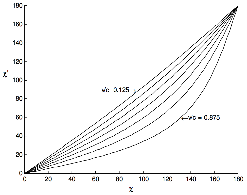
$\text{FIGURE XI.7}$

For Earth in orbit around the Sun, $v = 29.8 \ \text{km s}^{−1}$ and $v/c = 9.9 \times 10^{−5}$, which corresponds to an angle of $20^{\prime \prime} .5$. Thus the aberrational displacement is very small. If we write $ε = χ − χ^\prime$, Equation $\ref{11.3.8}$ takes the form to first order in $ε$:

$$\cos (χ - ε) = \cos χ + ε\sin χ = \frac{\cos χ + (v/c)}{1 + (v/c) \cos χ}, \label{11.3.10} \tag{11.3.10}$$

from which, after a very little algebra, we find

$$ε = \frac{(v/c) \sin χ}{1 + (v/c) χ}, \label{11.3.11} \tag{11.3.11}$$

or, since $v/c << 1,$

$$ε \approx \frac{v \sin χ}{c}, \label{11.3.12} \tag{11.3.12}$$

Thus we see that the aberrational displacement is zero at the apex and at the antapex, and it reaches is greatest value, $20^{\prime \prime} .5$, ninety degrees from the apex.

As with refraction, however, it is the differential aberration that counts, and if the diameter of the detector field is $δχ$, the difference $δε$ in the aberrational displacement across the field is

$$δε = \frac{v \cos χδχ}{c}. \label{11.3.13} \tag{11.3.13}$$

Notice that the differential aberration is greatest at the apex and antapex, and is zero ninety degrees from the apex. It might be noted that the opposition point, where perhaps the majority of asteroid observations are made, is ninety degrees from the apex.

The following table, similar to the one shown for differential refraction, shows the differential aberration across five-degree and 20-arcminute fields for various apical distances.

$$\begin{array}{c c c} \text{Apical distance} & δε \ \text{in arcseconds} & δε \ \text{in arcseconds} \\ \text{in degrees} & \text{for } 5^\circ \text{ field} & \text{for } 20^\prime \text{ field} \\ \\ 0 & 1.8 & 0.12 \\ 15 & 1.7 & 0.12 \\ 30 & 1.5 & 0.10 \\ 45 & 1.3 & 0.09 \\ 60 & 0.9 & 0.06 \\ 90 & 0.0 & 0.00 \\ \end{array}$$

It might be concluded that the effect of differential aberration is so small as to be scarcely worth worrying about in most circumstances. However, the expectations for the precision of asteroid astrometry are now rather stringent and are likely to become more exacting as time progresses, and for precise work the correction should be made. One of the problems with pre-packaged astrometry programs is that the user does not always know what corrections are included in the package. The surest way is to do it oneself.

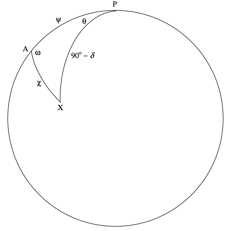
$\text{FIGURE XI.8}$

In figure $\text{XI.8}$, $\text{P}$ is the north celestial pole, $\text{A}$ is the apex of the Earth’s way, and $\text{X}$ is a star of true equatorial coordinates $(α , \delta)$. The apical distance $\text{AX}$ is $χ$. The angle θ is α(X) − α(A), the angle $\text{PAX}$ is $ω$, and $ψ$ is the distance from pole to apex. It is assumed that the observer knows how to calculate ω and ψ by the usual formulas of spherical astronomy, and hence that all angles in figure $\text{XI.8}$ are known.

From the cotangent formula, we have

$$\cos ψ \cos ω = \sin ψ \cot χ - \sin ω \cos θ . \label{11.3.14} \tag{11.3.14}$$

If $χ$ is increased by $δχ$, the corresponding increase in $θ$ is given by

$$\sin ω \sin θδθ = \sin ψ \csc^2 χδχ . \label{11.3.15} \tag{11.3.15}$$

Here $δθ = α^\prime (\text{X}) − α(\text{X})$, where $α$ and $α^\prime$ are, respectively, the true and apparent right ascensions of the star, and $δχ$ is $χ^\prime − χ$, which is $−ε$. It is easy to err in sign at this point, so I re-write Equation $\ref{11.3.15}$ more explicitly:

$$\left( α^\prime (X) - α(X) \right). \sin ω . \sin \left( α (X) - α (P) \right) = - ε \sin ψ \csc^2 χ . \label{11.3.16} \tag{11.3.16}$$

Here $ε$ is the aberrational displacement of $\text{X}$ towards $\text{A}$ given by Equation $\ref{11.3.12}$. On substitution of Equation $\ref{11.3.12}$ into Equation $\ref{11.3.16}$, this becomes, then,

$$\left( α^\prime (X) - α(X) \right) . \sin ω . \sin \left( α (X) - α (P) \right) = -\frac{v}{c} \sin ψ \csc χ. \label{11.3.17} \tag{11.3.17}$$

This enables us to calculate the apparent right ascension of the star.

The declination is obtained from an application of the cosine formula:

$$\sin \delta = \cos χ \cos ψ + \sin χ \sin ψ \cos ω, \label{11.3.18} \tag{11.3.18}$$

from which

$$\cos \delta δ \delta = \left( - \cos ψ \sin χ + \sin ψ \cos ω \cos χ \right) δχ. \label{11.3.19} \tag{11.3.19}$$

Here again, as in the usual convention of calculus, $δχ$ represents an increase in $χ$ and $δ \delta$ is the corresponding increase in $\delta$. But aberration results in a decrease of apical distance, so that $δχ = −ε$.

Equation 11.3.19 enables us to calculate the apparent declination of the star.

From the measurements of the positions of the comparison stars and the asteroid, we can now calculate the apparent right ascension and declination of the asteroid, and, by inversion of Equations $\ref{11.3.17}$ and 11.3.19, we can determine the true right ascension and declination of the asteroid.