10.2: Thermal Broadening

Let us start with an assumption that the radiation damping broadening is negligible, so that, for all practical purposes the spread of the frequencies emitted by a collection of atoms in a gas is infinitesimally narrow. The observer, however, will not see an infinitesimally thin line. This is because of the motion of the atoms in a hot gas. Some atoms are moving hither, and the wavelength will be blue-shifted; others are moving yon, and the wavelength will be red-shifted. The result will be a broadening of the lines, known as thermal broadening. The hotter the gas, the faster the atoms will be moving, and the broader the lines will be. We shall be able to measure the kinetic temperature of the gas from the width of the lines.

First, a brief reminder of the relevant results from the kinetic theory of gases, and to establish our notation.

$$\nonumber \begin{align}\text{Notation:}\qquad &c=\text{ speed of light } \\ \nonumber&\mathbf{V}=\text{ velocity of a particular atom }=u\hat{\mathbf{x}}+v\hat{\mathbf{y}}+w\hat{\mathbf{z}} \\ \nonumber &V = \text{ speed of that atom } = \left (u^2+v^2+w^2 \right )^{\frac{1}{2}} \\ \nonumber &V_\text{m} = \text{ modal speed of all the atoms } = \sqrt{\frac{2kT}{m}}=1.414\sqrt{\frac{kT}{m}} \\ \nonumber &\overline V = \text{mean speed of all the atoms }=\sqrt{\frac{8kT}{\pi m}}=1.596 \sqrt{\frac{kT}{m}}=1.128V_\text{m} \\ \nonumber &V_\text{RMS} =\text{ root mean square speed of all the atoms } =\sqrt{\frac{3kT}{m}}=1.732\sqrt{\frac{kT}{m}}=1.225V_\text{m} \\ \end{align}$$

The Maxwell distribution gives the distribution of speeds. Consider a gas of $N$ atoms, and let $N_VdV$ be the number of them that have speeds between $V\text{ and }V + dV$. Then

$$\label{10.3.1}\frac{N_VdV}{N}=\frac{4}{\sqrt{\pi}V_\text{m}^3}V^2\text{exp}\left ( -\frac{u^2}{V_\text{m}^2}\right ) dV.$$

More relevant to our present topic is the distribution of a velocity component. We’ll choose the $x$-component, and suppose that the $x$-direction is the line of sight of the observer as he or she peers through a stellar atmosphere. Let $N_udu$ be the number of atoms with velocity components between $u\text{ and }du$. Then the gaussian distribution is

$$\label{10.3.2}\frac{N_udu}{N}=\frac{1}{\sqrt{\pi}V_\text{m}}\text{exp}\left ( -\frac{u^2}{V_\text{m}^2}\right ) du,$$

which, of course, is symmetric about $u = 0$.

Now an atom with a line-of-sight velocity component $u$ gives rise to a Doppler shift $\nu - \nu_0$, where (provided that $u^2 << c^2$ ) $\frac{\nu-\nu_0}{\nu_0}=\frac{u}{c}$. If we are looking at an emission line, the left hand side of Equation $\ref{10.3.2}$ gives us the line profile $I_\nu(\nu)/I_\nu(\nu_0)$ (provided the line is optically thin, as is always assumed in this chapter unless specified otherwise). Thus the line profile of an emission line is

$$\label{10.3.3}\frac{I_\nu(\nu)}{I_\nu(\nu_0)}=\text{exp}\left [ -\frac{c^2}{V_\text{m}^2}\frac{(\nu-\nu_0)^2}{v\nu_0^2}\right ].$$

This is a gaussian, or Doppler, profile.

It is easy to show that the full width at half maximum (FWHM) is

$$\label{10.3.4}w=\frac{V_\text{m}\nu_0}{\text{c}}\sqrt{\ln 16}=1.6651\frac{V_\text{m}\nu_0}{\text{c}}.$$

This is also the full width at half minimum (FWHm) of an absorption line, in frequency units. This is also the FWHM or FWHm in wavelength units, provided that $\lambda_0$ be substituted for $\nu_0$.

The profile of an absorption line of central depth $d ( = \frac{I_\nu(\text{c})-I_\nu(\nu_0)}{I_\nu(\text{c})})$ is

$$\label{10.3.5}\frac{I_\nu(\nu)}{I_v(c)}=1-d\text{ exp}\left [ -\frac{c^2}{V_\text{m}^2}\frac{(\nu-\nu_0)^2}{\nu_0^2}\right ] ,$$

which can also be written

$$\label{10.3.6}\frac{I_\nu(\nu)}{I_\nu(\text{c})}=1-d \text{exp}\left [ -\frac{(\nu-\nu_0)^2\ln 16}{w^2}\right ].$$

(Verify that when $\nu - \nu_0 = \frac{1}{2}w$, the right hand side is $1-\frac{1}{2}d$. Do the same for equation 10.2.22.)

In figure X.2, I draw two gaussian profiles, each of the same equivalent width as the lorentzian profiles of figure X.1, and of the same two central depths, namely 0.4 and 0.8. We see that a gaussian profile is “all core and no wings”. A visual inspection of a profile may lead one to believe that it is probably gaussian, but, to be sure, one could write Equation $\ref{10.3.6}$ in the form

$$\label{10.3.7}\ln \left [ \frac{I_\nu(\text{c})-I_\nu(\nu)}{I_\nu(\text{c})}\right ] =\ln d -\frac{(\nu-\nu_0)^2\ln 16}{w^2}$$

and plot a graph of the left hand side versus $(\nu - \nu_0)^2$. If the profile is truly gaussian, this will result in a straight line, from which $w$ and $d$ can be found from the slope and intercept.

Integrating the Doppler profile to find the equivalent width is slightly less easy than integrating the Lorentz profile, but it is left as an exercise to show that

$$\nonumber \begin{align}\text{Equivalent width } &=\sqrt{\frac{\pi}{\ln 16}}\times\text{ central depth }\times \text{FWHm} \\ &=1.064 \times \text{ central depth }\times \text{FWHm}. \\ \end{align}$$

Compare this with equation 10.2.23 for a Lorentz profile.

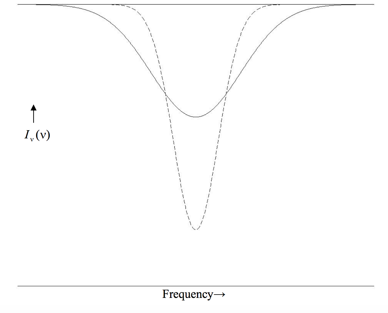
$\text{FIGURE X.2}$

Figure X.3 shows a lorentzian profile (continuous) and a gaussian profile (dashed), each having the same central depth and the same FWHm. The ratio of the lorenzian equivalent width to the gaussian equivalent width is $\frac{\pi}{2}\div \sqrt{\frac{\pi}{\ln 16}}=\sqrt{\pi \ln 2}=1.476.$

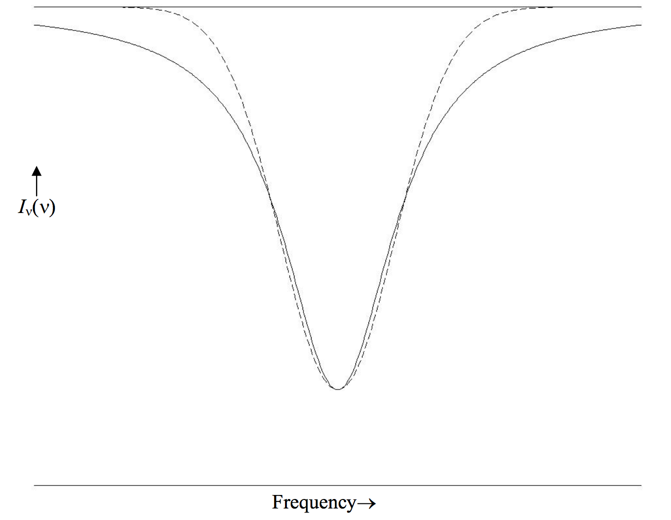
$\text{FIGURE X.3}$