
10.1: Natural Broadening (Radiation Damping)
- Page ID
- 6707

\( \newcommand{\vecs}[1]{\overset { \scriptstyle \rightharpoonup} {\mathbf{#1}} } \)
\( \newcommand{\vecd}[1]{\overset{-\!-\!\rightharpoonup}{\vphantom{a}\smash {#1}}} \)
\( \newcommand{\dsum}{\displaystyle\sum\limits} \)
\( \newcommand{\dint}{\displaystyle\int\limits} \)
\( \newcommand{\dlim}{\displaystyle\lim\limits} \)
\( \newcommand{\id}{\mathrm{id}}\) \( \newcommand{\Span}{\mathrm{span}}\)
( \newcommand{\kernel}{\mathrm{null}\,}\) \( \newcommand{\range}{\mathrm{range}\,}\)
\( \newcommand{\RealPart}{\mathrm{Re}}\) \( \newcommand{\ImaginaryPart}{\mathrm{Im}}\)
\( \newcommand{\Argument}{\mathrm{Arg}}\) \( \newcommand{\norm}[1]{\| #1 \|}\)
\( \newcommand{\inner}[2]{\langle #1, #2 \rangle}\)
\( \newcommand{\Span}{\mathrm{span}}\)
\( \newcommand{\id}{\mathrm{id}}\)
\( \newcommand{\Span}{\mathrm{span}}\)
\( \newcommand{\kernel}{\mathrm{null}\,}\)
\( \newcommand{\range}{\mathrm{range}\,}\)
\( \newcommand{\RealPart}{\mathrm{Re}}\)
\( \newcommand{\ImaginaryPart}{\mathrm{Im}}\)
\( \newcommand{\Argument}{\mathrm{Arg}}\)
\( \newcommand{\norm}[1]{\| #1 \|}\)
\( \newcommand{\inner}[2]{\langle #1, #2 \rangle}\)
\( \newcommand{\Span}{\mathrm{span}}\) \( \newcommand{\AA}{\unicode[.8,0]{x212B}}\)
\( \newcommand{\vectorA}[1]{\vec{#1}} % arrow\)
\( \newcommand{\vectorAt}[1]{\vec{\text{#1}}} % arrow\)
\( \newcommand{\vectorB}[1]{\overset { \scriptstyle \rightharpoonup} {\mathbf{#1}} } \)
\( \newcommand{\vectorC}[1]{\textbf{#1}} \)
\( \newcommand{\vectorD}[1]{\overrightarrow{#1}} \)
\( \newcommand{\vectorDt}[1]{\overrightarrow{\text{#1}}} \)
\( \newcommand{\vectE}[1]{\overset{-\!-\!\rightharpoonup}{\vphantom{a}\smash{\mathbf {#1}}}} \)
\( \newcommand{\vecs}[1]{\overset { \scriptstyle \rightharpoonup} {\mathbf{#1}} } \)
\(\newcommand{\longvect}{\overrightarrow}\)
\( \newcommand{\vecd}[1]{\overset{-\!-\!\rightharpoonup}{\vphantom{a}\smash {#1}}} \)
\(\newcommand{\avec}{\mathbf a}\) \(\newcommand{\bvec}{\mathbf b}\) \(\newcommand{\cvec}{\mathbf c}\) \(\newcommand{\dvec}{\mathbf d}\) \(\newcommand{\dtil}{\widetilde{\mathbf d}}\) \(\newcommand{\evec}{\mathbf e}\) \(\newcommand{\fvec}{\mathbf f}\) \(\newcommand{\nvec}{\mathbf n}\) \(\newcommand{\pvec}{\mathbf p}\) \(\newcommand{\qvec}{\mathbf q}\) \(\newcommand{\svec}{\mathbf s}\) \(\newcommand{\tvec}{\mathbf t}\) \(\newcommand{\uvec}{\mathbf u}\) \(\newcommand{\vvec}{\mathbf v}\) \(\newcommand{\wvec}{\mathbf w}\) \(\newcommand{\xvec}{\mathbf x}\) \(\newcommand{\yvec}{\mathbf y}\) \(\newcommand{\zvec}{\mathbf z}\) \(\newcommand{\rvec}{\mathbf r}\) \(\newcommand{\mvec}{\mathbf m}\) \(\newcommand{\zerovec}{\mathbf 0}\) \(\newcommand{\onevec}{\mathbf 1}\) \(\newcommand{\real}{\mathbb R}\) \(\newcommand{\twovec}[2]{\left[\begin{array}{r}#1 \\ #2 \end{array}\right]}\) \(\newcommand{\ctwovec}[2]{\left[\begin{array}{c}#1 \\ #2 \end{array}\right]}\) \(\newcommand{\threevec}[3]{\left[\begin{array}{r}#1 \\ #2 \\ #3 \end{array}\right]}\) \(\newcommand{\cthreevec}[3]{\left[\begin{array}{c}#1 \\ #2 \\ #3 \end{array}\right]}\) \(\newcommand{\fourvec}[4]{\left[\begin{array}{r}#1 \\ #2 \\ #3 \\ #4 \end{array}\right]}\) \(\newcommand{\cfourvec}[4]{\left[\begin{array}{c}#1 \\ #2 \\ #3 \\ #4 \end{array}\right]}\) \(\newcommand{\fivevec}[5]{\left[\begin{array}{r}#1 \\ #2 \\ #3 \\ #4 \\ #5 \\ \end{array}\right]}\) \(\newcommand{\cfivevec}[5]{\left[\begin{array}{c}#1 \\ #2 \\ #3 \\ #4 \\ #5 \\ \end{array}\right]}\) \(\newcommand{\mattwo}[4]{\left[\begin{array}{rr}#1 \amp #2 \\ #3 \amp #4 \\ \end{array}\right]}\) \(\newcommand{\laspan}[1]{\text{Span}\{#1\}}\) \(\newcommand{\bcal}{\cal B}\) \(\newcommand{\ccal}{\cal C}\) \(\newcommand{\scal}{\cal S}\) \(\newcommand{\wcal}{\cal W}\) \(\newcommand{\ecal}{\cal E}\) \(\newcommand{\coords}[2]{\left\{#1\right\}_{#2}}\) \(\newcommand{\gray}[1]{\color{gray}{#1}}\) \(\newcommand{\lgray}[1]{\color{lightgray}{#1}}\) \(\newcommand{\rank}{\operatorname{rank}}\) \(\newcommand{\row}{\text{Row}}\) \(\newcommand{\col}{\text{Col}}\) \(\renewcommand{\row}{\text{Row}}\) \(\newcommand{\nul}{\text{Nul}}\) \(\newcommand{\var}{\text{Var}}\) \(\newcommand{\corr}{\text{corr}}\) \(\newcommand{\len}[1]{\left|#1\right|}\) \(\newcommand{\bbar}{\overline{\bvec}}\) \(\newcommand{\bhat}{\widehat{\bvec}}\) \(\newcommand{\bperp}{\bvec^\perp}\) \(\newcommand{\xhat}{\widehat{\xvec}}\) \(\newcommand{\vhat}{\widehat{\vvec}}\) \(\newcommand{\uhat}{\widehat{\uvec}}\) \(\newcommand{\what}{\widehat{\wvec}}\) \(\newcommand{\Sighat}{\widehat{\Sigma}}\) \(\newcommand{\lt}{<}\) \(\newcommand{\gt}{>}\) \(\newcommand{\amp}{&}\) \(\definecolor{fillinmathshade}{gray}{0.9}\)The classical oscillator model of the atom was described in Section 9.2. In this model, the motion of the optical electron, when subject to the varying electromagnetic field of a light wave, obeys the differential equation for forced, damped, oscillatory motion:
\[\label{10.2.1}\ddot x+\gamma \dot x +\omega_0^2x=\frac{e\hat{E}}{m}\cos \omega t. \]
Because the oscillating (hence accelerating) electron itself radiates, the system loses energy, which is equivalent to saying that the motion is damped, and \(\gamma\) is the damping constant. Electromagnetic theory tell us that the rate of radiation of energy from an accelerating electron is
\[\label{10.2.2}\frac{2}{3}\cdot \frac{e^2\ddot x^2}{4\pi ε_0c^3}. \]
(The reader, as always, should check the dimensions of this and all subsequent expressions.)
For an electron that is oscillating, the average rate of loss of energy per cycle is
\[\label{10.2.3}\frac{2}{3}\cdot \frac{e^2 \overline{\ddot x^2}}{4\pi ε_0 c^3}. \]
Here the bar denotes the average value over a cycle.
If the amplitude and angular frequency of the oscillation are \(a\) and \(\omega_0\), the maximum acceleration is \(a\omega_0^2\) and the mean square acceleration is \(\frac{1}{2}a^2\omega_0^4\). The energy (kinetic plus potential) of the oscillating electron is
\[\label{10.2.4}W=\frac{1}{2}ma^2\omega_0^2. \]
Thus we can write for the average rate of loss per cycle of energy from the system by electromagnetic radiation:
\[\label{10.2.5}\frac{2}{3}\cdot\frac{e^2\omega_0^2}{4\pi ε_0 mc^3}\cdot W \]
The energy therefore falls off according to
\[\label{10.2.6}\dot W = -\frac{1}{3}\cdot \frac{e^2 \omega_0^2}{4\pi ε_0 mc^3}\cdot W. \]
The radiated wavelength is given by \(\lambda = 2\pi c /\omega_0\), so that Equation \ref{10.2.6} becomes
\[\dot W = -\frac{2\pi e^2}{3ε_0 mc \lambda^2}\cdot W.\label{10.2.7} \]
It will be recalled from the theory of lightly damped oscillations that the solution to Equation \ref{10.2.1} shows that the amplitude falls off with time as \(\text{exp}(-\frac{1}{2} \gamma t)\), and that the energy falls off as \(\text{exp}(-\gamma t)\). Thus we identify the coefficient of \(W\) on the right hand side of Equation \ref{10.2.7} as the classical radiation damping constant \(\gamma\):
\[\label{10.2.8}\gamma =\frac{2\pi e^2}{3ε_0mc\lambda^2}. \]
Numerically, if \(\gamma\) is in \(\text{s}^{-1}\) and \(\lambda\) is in \(\text{m}\),
\[\label{10.2.9}\gamma = \frac{2.223 \times 10^{-5}}{\lambda^2}. \]
We are now going to calculate the rate at which energy is transported per unit area by an electromagnetic wave, and also to calculate the rate at which an optically thin slab of a gas of classical oscillators absorbs energy, and hence we are going to calculate the classical absorption coefficient. We start by recalling, from elementary electromagnetism, that the energy held per unit volume in an electric field is \(\frac{1}{2}\textbf{D}\cdot \textbf{E}\) and the energy held per unit volume in a magnetic field is \(\frac{1}{2}\textbf{B}\cdot \textbf{H}\). In an isotropic medium, these become \(\frac{1}{2}ε E^2\) and \(\frac{1}{2}\mu H^2\), and, in vacuo, they become \(\frac{1}{2}ε_0E^2 \text{ and }\frac{1}{2}\mu_0H^2\).
For an oscillating electric field of the form \(E = \hat{E} \cos \omega t\), the average energy per unit volume per cycle is \(\frac{1}{2}ε_0 \overline{E^2} = \frac{1}{4}ε_0 \hat{E}^2\). Similarly for an oscillating magnetic field, the average energy per unit volume per cycle is \(\frac{1}{4}\mu_0 \hat{H}^2\). An electromagnetic wave consists of an electric and a magnetic wave moving at speed \(c\), so the rate at which energy is transmitted across unit area is \(\left ( \frac{1}{4}ε_0 \hat{E}^2+\frac{1}{4}\mu_0\hat{H}^2\right ) c\), and the two parts are equal, so that the rate at which energy is transmitted per unit area by a plane electromagnetic wave is \(\frac{1}{2}ε_0 \hat{E}^2c\).
Now we are modelling the classical oscillator as an electron bound to an atom, and being subject to a periodic force \(\frac{e\hat{E}}{m}\cos \omega t\) from an electromagnetic wave. The rate of absorption of energy by such an oscillator (see, for example, Chapter 12 of Classical Mechanics is
\[\frac{\gamma e^2 \hat{E}^2\omega^2}{2m[(\omega_0^2-\omega^2)^2+\gamma^2\omega^2]}.\nonumber \]
We imagine a plane electromagnetic wave arriving at (irradiating) a slab of gas containing \(\mathcal{N}\) classical oscillators per unit area, or \(n\) per unit volume. The rate of arrival of energy per unit area, we have seen, is \(\frac{1}{2}ε_0 \hat{E}^2c\). The rate of absorption of energy per unit area is
\[\frac{\mathcal{N}\gamma e^2\hat{E}^2\omega^2}{2m[(\omega_0^2-\omega^2)^2+\gamma^2\omega^2]}.\nonumber \]
The absorptance (see Chapter 2, section 2.2) is therefore
\[\label{10.2.10}a=\frac{\mathcal{N}\gamma e^2 \omega^2}{mε_0 c[(\omega_0^2-\omega^2)^2+\gamma^2\omega^2]}. \]
and the linear absorption coefficient is
\[\label{10.2.11}\alpha = \frac{n\gamma e^2 \omega^2}{mε_0 c[(\omega_0^2-\omega^2)^2+\gamma^2\omega^2]}. \]
A reminder here might be in order. Absorptance \(a\) is defined in section 2.2, and in the notation of figure IX.1, the absorptance at wavelength \(\lambda\) would be \(\left ( I_\lambda (c)-I_\lambda(\lambda)\right )/I_\lambda (c)\). Absorption coefficient \(\alpha\) is defined by equation 5.2.1: \(- dI/I = \alpha\,dx\). For a thick slice of gas, of thickness \(t\), this integrates, in the notation of figure IX.1, to \(I_\lambda (\lambda)= I_\lambda (c) \text{exp}(-\alpha t)\). But for an optically thin gas, which is what we are considering, unless stated otherwise, in this chapter, this becomes \(\left ( I_\lambda (c) - I_\lambda (\lambda)\right )/ I_\lambda (c) = \alpha t\). Thus, for an optically thin gas, absorptance is just absorption coefficient times thickness of the gas. And the relation between particle density \(n\) and column density \(\mathcal{N}\text{ is }\mathcal{N} = nt\).
We can write \(\omega_0^2 -\omega = \left ( \omega_0 -\omega \right ) \left ( \omega_0 + \omega \right )\). Let us also write \(\omega\) as \(2\pi ν\). Also, in the near vicinity of the line, let us make the approximation \(\omega_0 + \omega = 2\omega\). We then obtain for the absorption coefficient, in the vicinity of the line,
\[\label{10.2.12}\alpha = \frac{\gamma n e^2}{16\pi^2 mcε_0 \left [ (\nu-\nu_0)^2+\left ( \frac{\gamma }{4\pi}\right )^2\right ]} . \]
Make sure that I have made no mistakes in deriving equations \ref{10.2.10},11 and 12, and check the dimensions of each expression as you go. Let me know if you find anything wrong.
Now the equivalent width in frequency units of an absorption line in an optically thin layer of gas of geometric thickness \(t\) is (see equation 9.1.6)
\[\label{10.2.13}W^{(\nu)}=t\int_{-\infty}^\infty \alpha d(\nu-\nu_0). \]
(a) For those readers who (understandably) object that expression \ref{10.2.12} is valid only in the immediate vicinity of the line, and therefore that we cannot integrate from \(-\infty \text{ to }+\infty\), integrate expression \ref{10.2.11} from \(0\text{ to }\infty\).
(b) For the rest of us, integrate Equation \ref{10.2.11} from \(ν - ν_0 = -\infty\text{ to }+ \infty\). A substitution \(4\pi (ν - ν_0 ) = \gamma \tan \theta\) will probably be a good start.
We obtain
\[\label{10.2.14}W^{(\nu)}=\frac{\mathcal{N}e^2}{4mcε_0}=2.654\times 10^{-6}\mathcal{N}, \]
where \(W^{(\nu)}\) is in \(\text{Hz}\) and \(\mathcal{N}\) is in \(\text{m}^{-2}\). Thus the classical oscillator model predicts that the equivalent width in frequency units is independent of the frequency (and hence wavelength) of the line, and also independent of the damping constant. If we express the equivalent width in wavelength units (see equation 9.1.3), we obtain:
\[\label{10.2.15}W=\frac{\mathcal{N}e^2\lambda^2}{4mc^2ε_0}. \]
This is the same as equation 9.2.2.
When we discussed this equation in Chapter 9, we pointed out that the equivalent widths of real lines differ from this prediction by a factor \(f_{12}\), the absorption oscillator strength, and we also pointed out that \(\mathcal{N}\) has to be replaced by \(\mathcal{N}_1\), the column density of atoms in the initial (lower) level. Thus, from this point, I shall replace \(\mathcal{N}\) with \(\mathcal{N}_1f_{12}\). However, in this chapter we are not so much concerned with the equivalent width, but with the line profile and the actual width. The width of an emission line in this context is commonly expressed as the full width at half maximum (FWHM) and the width of an absorption line as the full width at half minimum (FWHm). (These are on no account to be confused with the equivalent width, which is discussed in section 9.1.) Note that some writers use the term “half-width”. It is generally not possible to know what a writer means by this.
In terms of the notation of figure IX.1 (in which “\(\text{c}\)” denotes “continuum”), but using a frequency rather than a wavelength scale, the absorptance at frequency \(ν\) is
\[\label{10.2.16}a(\nu)=\frac{I_\nu(\text{c})-I_\nu(\nu)}{I_\nu(\text{c})}. \]
The profile of an absorption line is thus given by
\[\label{10.2.17}I_\nu(\nu)=I_\nu(\text{c})\left (1-a(\nu)\right ). \]
For radiation damping we have
\[\label{10.2.18}a(\nu)=\frac{\gamma \mathcal{N}_1 f_{12}e^2}{16\pi^2mcε_0\left [ (\nu-\nu_0)^2+\left ( \frac{\gamma}{4\pi}\right )^2\right ] }. \]
The maximum value of the absorptance (at the line centre) is
\[\label{10.2.19}a(\nu_0)=\frac{\mathcal{N}_1f_{12}e^2}{mcε_0 \gamma}. \]
This quantity is also \(\frac{I_\nu(\text{c})-I_\nu(\nu_0)}{I_\nu(\text{c})}\) and it is also known as the central depth \(d\) of the line. (Be sure to refer to figure IX.1 to understand its meaning.) I shall use the symbol \(d\text{ or }a(\nu_0)\) interchangeably, according to context.
It is easy to see that the value of \(\nu-\nu_0\) at which the absorptance is half its maximum value is \(\gamma /(4\pi)\). That is to say, the full width at half maximum (FWHM) of the absorptance, which I denote as \(w\), is, in frequency units:
\[\label{10.2.20}w=\frac{\gamma}{2\pi}. \]
(In wavelength units, it is \(\lambda^2 /c\) times this.) This is also the FWHM of the absorption profile.
Equation \ref{10.2.18} can be written
\[\label{10.2.21}\frac{a(\nu)}{a(\nu_0)}=\frac{1}{4\left ( \frac{\nu-\nu_0}{w}\right )^2+1}. \]
The absorption line profile (see Equation \ref{10.2.1}) can be written
\[\label{10.2.22}\frac{I_\nu(\nu)}{I_\nu(\text{c})}=1-\frac{d}{4\left ( \frac{\nu-\nu_0}{w}\right )^2+1}. \]
Notice that at the line centre, \(I_\nu(\nu_0)/I_\nu(\text{c}) = 1\) minus the central depth; and a long way from the line centre, \(I_\nu(\nu) = I_\nu(\text{c})\), as expected. This type of profile is called a Lorentz profile.
From equations \ref{10.2.14} (but with \(\mathcal{N}_1f_{12}\) substituted for \(\mathcal{N}\)), \ref{10.2.19} and \ref{10.2.20}, we find that
\[\nonumber \begin{align}\text{Equivalent width}&=\frac{\pi}{2}\times\text{ central depth }\times\text{ FWHm} \\ &1.571\times \text{ central depth }\times \text{ FWHm}. \\ \end{align} \nonumber \]
This is true whether equivalent width and FWHm are measured in frequency or in wavelength units. (It is a pity that, for theoretical work, frequency is more convenient than wavelength, since frequency is proportional to energy, but experimentalists often (not invariably!) work with gratings, which disperse light linearly with respect to wavelength!)
Indeed the equivalent width of any type of profile can be written in the form
\[\label{10.2.24}\text{Equivalent width }=\text{ constant }\times\text{ central depth }\times\text{ FWHm }, \]
the value of the constant depending upon the type of profile.
In photographic days, the measurement of equivalent widths was a very laborious procedure, and, if one had good reason to believe that the line profiles in a spectrum were all lorentzian, the equivalent with would be found by measuring just the FWHm and the central depth. Even today, when equivalent widths can often be determined by computer from digitally-recorded spectra almost instantaneously, there may be occasions where low-resolution spectra do not allow this, and all that can be honestly measured are the central depths and equivalent widths. The type of profile, and hence the value to be used for the constant in Equation \ref{10.2.14}, requires a leap of faith.
It is worth noting (consult equations \ref{10.2.4},\ref{10.2.19} and \ref{10.2.20}) that the equivalent width is determined by the column density of the absorbing atoms (or, rather, on \(\mathcal{N}_1f_{12}\)), the FWHm is determined by the damping constant, but the central depth depends on both. You can determine the damping constant by measuring the FWHm.
The form of the Lorentz profile is shown in figure X.1 for two lines, one with a central depth of 0.8 and the other with a central depth of 0.4. Both lines have the same equivalent width, the product \(wd\) being the same for each. Note that this type of profile has a narrow core, skirted by extensive wings.
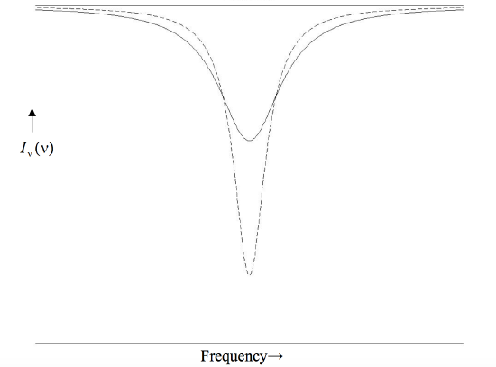
\(\text{FIGURE X.1}\)
Of course a visual inspection of a profile showing a narrow core and extensive wings, while suggestive, doesn’t prove that the profile is strictly lorentzian. However, Equation \ref{10.2.22} can be rearranged to read
\[\label{10.2.25}\frac{I_\nu(\text{c})}{I_\nu(\text{c})-I_\nu(\nu)}=\frac{4}{w^2d}\left (\nu-\nu_0 \right )^2+\frac{1}{d^2}. \]
This shows that if you make a series of measurements of \(I_ν(ν)\) and plot a graph of the left hand side versus \((ν-ν_0)^2\), you should obtain a straight line if the profile is lorentzian, and you will obtain the central depth and equivalent width (hence also the damping constant and the column density) from the intercept and slope as a bonus. And if you don’t get a straight line, you don’t have a Lorentz profile.
It will be recalled that the purely classical oscillator theory predicted that the equivalent widths of all lines (in frequency units) of a given element is the same, namely that given by Equation \ref{10.2.14}. The obvious observation that this is not so led us to introduce the emission oscillator strength, and also to replace \(\mathcal{N}\text{ by }\mathcal{N}_1\). Likewise, Equation \ref{10.2.20} predicts that the FWHm (in wavelength units) is the same for all lines. (Equation 10.2.20 gives the FWHm in frequency units. To understand my caveat “in wavelength units”, refer also to equations \ref{10.2.8} and \ref{10.2.9}. You will see that the predicted FWHm in wavelength units is \(\frac{e^2}{3\epsilon_0mc^2}=1.18\times 10^{-14}\text{m}\), which is exceedingly small, and the core, at least, is beyond the resolution of most spectrographs.) Obviously the damping constants for real lines are much larger than this. For real lines, the classical damping constant \(\gamma\) has to be replaced with the quantum mechanical damping constant \(\Gamma\).
At present I am describing in only a very qualitative way the quantum mechanical treatment of the damping constant. Quantum mechanically, an electromagnetic wave is treated as a perturbation to the hamiltonian operator. We have seen in section 9.4 that each level has a finite lifetime – see especially equation 9.4.7. The mean lifetime for a level \(m\text{ is }1/\Gamma_m\). Each level is not infinitesimally narrow. That is to say, one cannot say with infinitesimal precision what the energy of a given level (or state) is. The uncertainty of the energy and the mean lifetime are related through Heisenberg’s uncertainty principle. The longer the lifetime, the broader the level. The energy probability of a level \(m\) is given by a Lorentz function with parameter \(\Gamma_m\), given by equation 9.4.7 and equal to the reciprocal of the mean lifetime. Likewise a level \(n\) has an energy probability distribution given by a Lorentz function with parameter \(\Gamma_n\). When an atom makes a transition between \(m\text{ and }n\), naturally, there is an energy uncertainty in the emitted or absorbed photon, and so there is a distribution of photons (i.e. a line profile) that is a Lorentz function with parameter \(\Gamma = \Gamma_m + \Gamma_n\). This parameter \(\Gamma\) must replace the classical damping constant \(\gamma\). The FWHm of a line, in frequency units, is now \(\Gamma/(2\pi)\), which varies from line to line.
Unfortunately it is observed, at least in the spectrum of main sequence stars, if not in that of giants and supergiants, that the FWHms of most lines are about the same! How frustrating! Classical theory predicts that all lines have the same FWHm. We know classical theory is wrong, so we go to the trouble of doing quantum mechanical theory, which predicts different FWHms from line to line. And then we go and observe main sequence stars and we find that the lines all have the same FWHm (admittedly much broader than predicted by classical theory.)
The explanation is that, in main sequence atmospheres, lines are additionally broadened by pressure broadening, which also gives a Lorentz profile, which is generally broader than, and overmasks, radiation damping. (The pressures in the extended atmospheres of giants and supergiants are generally much less than in main sequence stars, and consequently lines are narrower.) We return to pressure broadening in a later section.