11.6: Curve of Growth for Voigt Profiles

Our next task is to construct curves of growth for Voigt profiles for different values of the ratio of the lorentzian and gaussian HWHMs, $l/g$, which is

$$\tag{11.6.1}\label{11.6.1}\frac{l}{g}=\frac{\Gamma \lambda_0}{4\pi V_\text{m}\sqrt{\ln 2}}=\frac{\Gamma \lambda_0}{V_\text{m}\pi \sqrt{\ln 65536}}=\frac{\Gamma \lambda_0}{34.841V_\text{m}},$$

or, better, for different values of the gaussian ratio $k_G =\frac{g}{l+g}$. These should look intermediate in appearance between figures XI.3 and 5.

The expression for the equivalent width in wavelength units is given by Equation 11.3.4:

$$\tag{11.3.4}\label{11.3.4}W=2\int_0^\infty \left [ 1-\text{exp}\left \{ -\tau(x)\right \}\right ]\,dx.$$

combined with Equation 10.5.20

$$\tag{10.5.20}\label{10.5.20}\tau (x) = Cl \tau (0)\int_{-\infty}^\infty \frac{\text{exp}\left [ -(ξ-x)^2\ln 2/g^2\right ]}{ξ^2+l^2}\,dξ.$$

That is:

$$\tag{11.6.2}\label{11.6.2}W=2\int_0^\infty \left ( 1-\text{exp} \left \{ -Cl\tau(0)\int_{-\infty}^\infty \frac{\text{exp}\left [ -(ξ-x)^2\ln 2/g^2 \right ]}{ξ^2+l^2}dξ\right \}\right )\,dx.$$

Here

• $x = \lambda − \lambda_0$, $l$ is the Lorentzian $\text{HWHM} = \lambda_0^2\Gamma/(4\pi c)$ (where $\Gamma$ may include a pressure-broadening contribution),
• $g$ is the gaussian $\text{HWHM} = V_\text{m}\lambda_0\sqrt{\ln 2} / c$ (where $V_\text{m}$ may include a microturbulence contribution), and
• $W$ is the equivalent width, all of dimension $L$.

The symbol $ξ$, also of dimension L, is a dummy variable, which disappears after the definite integration. $\tau(0)$ is the optical thickness at the line centre. $C$ is a dimensionless number given by Equation 10.5.23 and tabulated as a function of gaussian fraction in Chapter 10. The reader is urged to check the dimensions of Equation $\ref{11.6.2}$ carefully. The integration of Equation $\ref{11.6.2}$ is discussed in Appendix A.

Our aim is to calculate the equivalent width as a function of $\tau(0)$ for different values of the gaussian fraction $k_G = g/(l + g)$. What we find is as follows. Let $W^\prime = W \sqrt{\ln 2 }/g$; that is, $W^\prime$ is the equivalent width expressed in units of $g /\sqrt{ \ln 2}$. For $\tau(0)$ less than about 5, where the wings contribute relatively little to the equivalent width, we find that $W^\prime$ is almost independent of the gaussian fraction. The difference in behaviour of the curve of growth for different profiles appears only for large values of $\tau (0)$, when the wings assume a larger role. However, for any profile which is less gaussian than about $k_G$ equal to about 0.9, the behaviour of the curve of growth (for $\tau(0) > 5$) mimics that for a lorentzian profile. For that reason I have drawn curves of growth in figure XI.6 only for $k_G = 0.9, 0.99, 0.999\text{ and }1$. This corresponds to $l/g = 0.1111, 0.0101, 0.0010\text{ and }0$, or to $\Gamma \lambda_0 /V_m = 1.162, 0.1057, 0.0105\text{ and }0$ respectively.

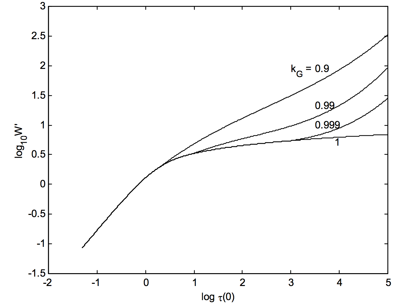
$\text{FIGURE XI.6}$