Physics LibreTexts

11.6: Curve of Growth for Voigt Profiles

  • Page ID
    6718
  • \( \newcommand{\vecs}[1]{\overset { \scriptstyle \rightharpoonup} {\mathbf{#1}} } \)

    \( \newcommand{\vecd}[1]{\overset{-\!-\!\rightharpoonup}{\vphantom{a}\smash {#1}}} \)

    \( \newcommand{\id}{\mathrm{id}}\) \( \newcommand{\Span}{\mathrm{span}}\)

    ( \newcommand{\kernel}{\mathrm{null}\,}\) \( \newcommand{\range}{\mathrm{range}\,}\)

    \( \newcommand{\RealPart}{\mathrm{Re}}\) \( \newcommand{\ImaginaryPart}{\mathrm{Im}}\)

    \( \newcommand{\Argument}{\mathrm{Arg}}\) \( \newcommand{\norm}[1]{\| #1 \|}\)

    \( \newcommand{\inner}[2]{\langle #1, #2 \rangle}\)

    \( \newcommand{\Span}{\mathrm{span}}\)

    \( \newcommand{\id}{\mathrm{id}}\)

    \( \newcommand{\Span}{\mathrm{span}}\)

    \( \newcommand{\kernel}{\mathrm{null}\,}\)

    \( \newcommand{\range}{\mathrm{range}\,}\)

    \( \newcommand{\RealPart}{\mathrm{Re}}\)

    \( \newcommand{\ImaginaryPart}{\mathrm{Im}}\)

    \( \newcommand{\Argument}{\mathrm{Arg}}\)

    \( \newcommand{\norm}[1]{\| #1 \|}\)

    \( \newcommand{\inner}[2]{\langle #1, #2 \rangle}\)

    \( \newcommand{\Span}{\mathrm{span}}\) \( \newcommand{\AA}{\unicode[.8,0]{x212B}}\)

    \( \newcommand{\vectorA}[1]{\vec{#1}}      % arrow\)

    \( \newcommand{\vectorAt}[1]{\vec{\text{#1}}}      % arrow\)

    \( \newcommand{\vectorB}[1]{\overset { \scriptstyle \rightharpoonup} {\mathbf{#1}} } \)

    \( \newcommand{\vectorC}[1]{\textbf{#1}} \)

    \( \newcommand{\vectorD}[1]{\overrightarrow{#1}} \)

    \( \newcommand{\vectorDt}[1]{\overrightarrow{\text{#1}}} \)

    \( \newcommand{\vectE}[1]{\overset{-\!-\!\rightharpoonup}{\vphantom{a}\smash{\mathbf {#1}}}} \)

    \( \newcommand{\vecs}[1]{\overset { \scriptstyle \rightharpoonup} {\mathbf{#1}} } \)

    \( \newcommand{\vecd}[1]{\overset{-\!-\!\rightharpoonup}{\vphantom{a}\smash {#1}}} \)

    \(\newcommand{\avec}{\mathbf a}\) \(\newcommand{\bvec}{\mathbf b}\) \(\newcommand{\cvec}{\mathbf c}\) \(\newcommand{\dvec}{\mathbf d}\) \(\newcommand{\dtil}{\widetilde{\mathbf d}}\) \(\newcommand{\evec}{\mathbf e}\) \(\newcommand{\fvec}{\mathbf f}\) \(\newcommand{\nvec}{\mathbf n}\) \(\newcommand{\pvec}{\mathbf p}\) \(\newcommand{\qvec}{\mathbf q}\) \(\newcommand{\svec}{\mathbf s}\) \(\newcommand{\tvec}{\mathbf t}\) \(\newcommand{\uvec}{\mathbf u}\) \(\newcommand{\vvec}{\mathbf v}\) \(\newcommand{\wvec}{\mathbf w}\) \(\newcommand{\xvec}{\mathbf x}\) \(\newcommand{\yvec}{\mathbf y}\) \(\newcommand{\zvec}{\mathbf z}\) \(\newcommand{\rvec}{\mathbf r}\) \(\newcommand{\mvec}{\mathbf m}\) \(\newcommand{\zerovec}{\mathbf 0}\) \(\newcommand{\onevec}{\mathbf 1}\) \(\newcommand{\real}{\mathbb R}\) \(\newcommand{\twovec}[2]{\left[\begin{array}{r}#1 \\ #2 \end{array}\right]}\) \(\newcommand{\ctwovec}[2]{\left[\begin{array}{c}#1 \\ #2 \end{array}\right]}\) \(\newcommand{\threevec}[3]{\left[\begin{array}{r}#1 \\ #2 \\ #3 \end{array}\right]}\) \(\newcommand{\cthreevec}[3]{\left[\begin{array}{c}#1 \\ #2 \\ #3 \end{array}\right]}\) \(\newcommand{\fourvec}[4]{\left[\begin{array}{r}#1 \\ #2 \\ #3 \\ #4 \end{array}\right]}\) \(\newcommand{\cfourvec}[4]{\left[\begin{array}{c}#1 \\ #2 \\ #3 \\ #4 \end{array}\right]}\) \(\newcommand{\fivevec}[5]{\left[\begin{array}{r}#1 \\ #2 \\ #3 \\ #4 \\ #5 \\ \end{array}\right]}\) \(\newcommand{\cfivevec}[5]{\left[\begin{array}{c}#1 \\ #2 \\ #3 \\ #4 \\ #5 \\ \end{array}\right]}\) \(\newcommand{\mattwo}[4]{\left[\begin{array}{rr}#1 \amp #2 \\ #3 \amp #4 \\ \end{array}\right]}\) \(\newcommand{\laspan}[1]{\text{Span}\{#1\}}\) \(\newcommand{\bcal}{\cal B}\) \(\newcommand{\ccal}{\cal C}\) \(\newcommand{\scal}{\cal S}\) \(\newcommand{\wcal}{\cal W}\) \(\newcommand{\ecal}{\cal E}\) \(\newcommand{\coords}[2]{\left\{#1\right\}_{#2}}\) \(\newcommand{\gray}[1]{\color{gray}{#1}}\) \(\newcommand{\lgray}[1]{\color{lightgray}{#1}}\) \(\newcommand{\rank}{\operatorname{rank}}\) \(\newcommand{\row}{\text{Row}}\) \(\newcommand{\col}{\text{Col}}\) \(\renewcommand{\row}{\text{Row}}\) \(\newcommand{\nul}{\text{Nul}}\) \(\newcommand{\var}{\text{Var}}\) \(\newcommand{\corr}{\text{corr}}\) \(\newcommand{\len}[1]{\left|#1\right|}\) \(\newcommand{\bbar}{\overline{\bvec}}\) \(\newcommand{\bhat}{\widehat{\bvec}}\) \(\newcommand{\bperp}{\bvec^\perp}\) \(\newcommand{\xhat}{\widehat{\xvec}}\) \(\newcommand{\vhat}{\widehat{\vvec}}\) \(\newcommand{\uhat}{\widehat{\uvec}}\) \(\newcommand{\what}{\widehat{\wvec}}\) \(\newcommand{\Sighat}{\widehat{\Sigma}}\) \(\newcommand{\lt}{<}\) \(\newcommand{\gt}{>}\) \(\newcommand{\amp}{&}\) \(\definecolor{fillinmathshade}{gray}{0.9}\)

    Our next task is to construct curves of growth for Voigt profiles for different values of the ratio of the lorentzian and gaussian HWHMs, \(l/g\), which is

    \[\tag{11.6.1}\label{11.6.1}\frac{l}{g}=\frac{\Gamma \lambda_0}{4\pi V_\text{m}\sqrt{\ln 2}}=\frac{\Gamma \lambda_0}{V_\text{m}\pi \sqrt{\ln 65536}}=\frac{\Gamma \lambda_0}{34.841V_\text{m}},\]

    or, better, for different values of the gaussian ratio \(k_G =\frac{g}{l+g}\). These should look intermediate in appearance between figures XI.3 and 5.

    The expression for the equivalent width in wavelength units is given by Equation 11.3.4:

    \[\tag{11.3.4}\label{11.3.4}W=2\int_0^\infty \left [ 1-\text{exp}\left \{ -\tau(x)\right \}\right ]\,dx.\]

    combined with Equation 10.5.20

    \[\tag{10.5.20}\label{10.5.20}\tau (x) = Cl \tau (0)\int_{-\infty}^\infty \frac{\text{exp}\left [ -(ξ-x)^2\ln 2/g^2\right ]}{ξ^2+l^2}\,dξ.\]

    That is:

    \[\tag{11.6.2}\label{11.6.2}W=2\int_0^\infty \left ( 1-\text{exp} \left \{ -Cl\tau(0)\int_{-\infty}^\infty \frac{\text{exp}\left [ -(ξ-x)^2\ln 2/g^2 \right ]}{ξ^2+l^2}dξ\right \}\right )\,dx.\]

    Here

    • \(x = \lambda − \lambda_0\), \(l\) is the Lorentzian \(\text{HWHM} = \lambda_0^2\Gamma/(4\pi c)\) (where \(\Gamma\) may include a pressure-broadening contribution),
    • \(g\) is the gaussian \(\text{HWHM} = V_\text{m}\lambda_0\sqrt{\ln 2} / c\) (where \(V_\text{m}\) may include a microturbulence contribution), and
    • \(W\) is the equivalent width, all of dimension \(L\).

    The symbol \(ξ\), also of dimension L, is a dummy variable, which disappears after the definite integration. \(\tau(0)\) is the optical thickness at the line centre. \(C\) is a dimensionless number given by Equation 10.5.23 and tabulated as a function of gaussian fraction in Chapter 10. The reader is urged to check the dimensions of Equation \ref{11.6.2} carefully. The integration of Equation \ref{11.6.2} is discussed in Appendix A.

    Our aim is to calculate the equivalent width as a function of \(\tau(0)\) for different values of the gaussian fraction \(k_G = g/(l + g)\). What we find is as follows. Let \(W^\prime = W \sqrt{\ln 2 }/g\); that is, \(W^\prime\) is the equivalent width expressed in units of \(g /\sqrt{ \ln 2}\). For \(\tau(0)\) less than about 5, where the wings contribute relatively little to the equivalent width, we find that \(W^\prime\) is almost independent of the gaussian fraction. The difference in behaviour of the curve of growth for different profiles appears only for large values of \(\tau (0)\), when the wings assume a larger role. However, for any profile which is less gaussian than about \(k_G\) equal to about 0.9, the behaviour of the curve of growth (for \(\tau(0) > 5\)) mimics that for a lorentzian profile. For that reason I have drawn curves of growth in figure XI.6 only for \(k_G = 0.9, 0.99, 0.999\text{ and }1\). This corresponds to \(l/g = 0.1111, 0.0101, 0.0010\text{ and }0\), or to \(\Gamma \lambda_0 /V_m = 1.162, 0.1057, 0.0105\text{ and }0\) respectively.

    alt
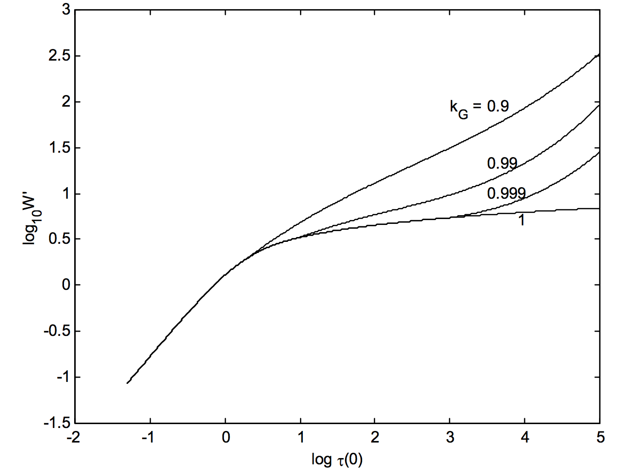
    \(\text{FIGURE XI.6}\)


    This page titled 11.6: Curve of Growth for Voigt Profiles is shared under a CC BY-NC 4.0 license and was authored, remixed, and/or curated by Jeremy Tatum via source content that was edited to the style and standards of the LibreTexts platform.