2.1: The Straight Line

It might be thought that there is rather a limited amount that could be written about the geometry of a straight line. We can manage a few Equations here, however, (there are 35 in this section on the Straight Line) and we shall return for more on the subject in Chapter 4.

Most readers will be familiar with the Equation for a straight line:

\[y = mx + c \label{2.2.1} \tag{2.2.1}\]

The slope (or gradient) of the line, which is the tangent of the angle that it makes with the \(x\)-axis, is \(m\), and the intercept on the \(y\)-axis is \(c\). There are various other forms that may be of use, such as

\[\frac{x}{x_0} + \frac{y}{y_0} = 1 \label{2.2.2} \tag{2.2.2}\]

\[\frac{y-y_1}{x-x_1} = \frac{y_2-y_1}{x_2-x_1} \label{2.2.3} \tag{2.2.3}\]

which can also be written

\begin{array}{| c c c | c}
x & y & 1 \\
x_1 & y_1 & 1 & =0 \\
x_2 & y_2 & 1 \\
\label{2.2.4} \tag{2.2.4}
\end{array}

\[x \cos \theta + y \sin \theta = p \label{2.25} \tag{2.2.5}\]

The four forms are illustrated in figure \(\text{II.1}\).

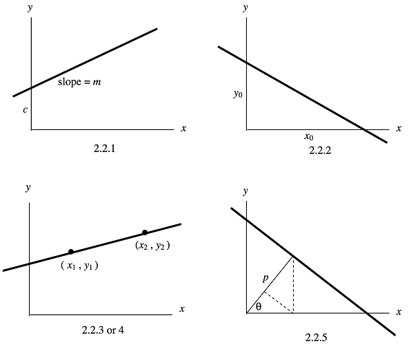
\(\text{FIGURE II.1}\)

A straight line can also be written in the form

\[Ax + By + C = 0. \label{2.2.6} \tag{2.2.6}\]

If \(C = 0\), the line passes through the origin. If \(C ≠ 0\), no information is lost, and some arithmetic and algebra are saved, if we divide Equation \ref{2.2.6} by \(C\) and re-write it in the form

\[ax + by = 1. \label{2.2.7} \tag{2.2.7}\]

Let \(P (x , y)\) be a point on the line and let \(P_0 (x_0 , y_0 )\) be a point in the plane not necessarily on the line. It is of interest to find the perpendicular distance between \(P_0\) and the line. Let \(S\) be the square of the distance between \(P_0\) and \(P\). Then

\[S = (x-x_0)^2 + (y-y_0)^2 \label{2.2.8} \tag{2.2.8}\]

We can express this in terms of the single variable \(x\) by substitution for \(y\) from Equation \(\ref{2.2.7}\). Differentiation of \(S\) with respect to \(x\) will then show that \(S\) is least for

\[x = \frac{a+b(bx_0 - ay_0)}{a^2 + b^2} \label{2.2.9} \tag{2.2.9}\]

The corresponding value for \(y\), found from Equations \(\ref{2.2.7}\) and \(\ref{2.2.9}\), is

\[y = \frac{b+a(ay_0 - bx_0)}{a^2 + b^2}. \label{2.2.10} \tag{2.2.10}\]

The point \(\text{P}\) described by Equations \(\ref{2.2.9}\) and \(\ref{2.2.10}\) is the closest point to \(\text{P}_0\) on the line. The perpendicular distance of \(\text{P}\) from the line is \(p = √S\) or

\[p = \frac{1-ax_0 - by_0}{\sqrt{a^2+b^2}}. \label{2.2.11} \tag{2.2.11}\]

This is positive if \(\text{P}_0\) is on the same side of the line as the origin, and negative if it is on the opposite side. If the perpendicular distances of two points from the line, as calculated from Equation \(\ref{2.2.11}\), are of opposite signs, they are on opposite sides of the line. If \(p = 0\), or indeed if the numerator of Equation \(\ref{2.2.11}\) is zero, the point \(\text{P}_0 (x_0 , y_0 )\) is, of course, on the line.

Let \(\text{A}(x_1 , y_1 ), \ \text{B}(x_2 , y_2 )\) and \(\text{C}(x_3 , y_3 )\) be three points in the plane. What is the area of the triangle \(\text{ABC}\)? One way to answer this is suggested by figure \(\text{II.2}\).

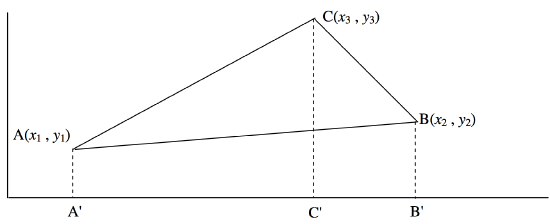
\(\text{FIGURE II.2}\)

We see that

area of triangle \(\text{ABC}\) = area of trapezium \(\text{A}^\prime \text{ACC}^\prime\) (see comment*)
+ area of trapezium \(\text{C}^\prime \text{CBB}^\prime\)
− area of trapezium \(\text{A}^\prime \text{ABB}^\prime\).

\[ = \frac{1}{2} (x_3 - x_1) (y_3 + y_1) + \frac{1}{2} (x_2 - x_3)(y_2 + y_3) - \frac{1}{2} (x_2 - x_1) (y_2 + y_1) \]
\[ = \frac{1}{2} [x_1(y_2 - y_3) + x_2 (y_3 -y_1) + x_3(y_1 - y_2)]\]

\begin{array}{l r | c c c |}
& & x_1 & x_2 & x_3 \\
= & \frac{1}{2} & y_1 & y_2 & y_3 \\
& & 1 & 1 & 1 \\
\label{2.2.12} \tag{2.2.12}
\end{array}

* Since writing this section I have become aware of a difference in U.S./British usages of the word "trapezium". Apparently in British usage, "trapezium" means a quadrilateral with two parallel sides. In U.S. usage, a trapezium means a quadrilateral with no parallel sides, while a quadrilateral with two parallel sides is a "trapezoid". As with many words, either British or U.S. usages may be heard in Canada. In the above derivation, I intended the British usage. What is to be learned from this is that we must always take care to make ourselves clearly understood when using such ambiguous words, and not to assume that the reader will interpret them the way we intend.

The reader might like to work through an alternative method, using results that we have obtained earlier. The same result will be obtained. In case the algebra proves a little tedious, it may be found easier to work through a numerical example, such as: calculate the area of the triangle \(\text{ABC}\), where \(\text{A}\), \(\text{B}\), \(\text{C}\) are the points (2,3), (7,4), (5,6) respectively. In the second method, we note that the area of a triangle is \(\frac{1}{2} \times \text{base} \times \text{height}\). Thus, if we can find the length of the side BC, and the perpendicular distance of \(\text{A}\) from \(\text{BC}\), we can do it. The first is easy:

\[(\text{BC})^2 = (x_3 - x_2)^2 + (y_3 - y_2)^2 . \label{2.2.13} \tag{2.2.13}\]

To find the second, we can easily write down the Equation to the line \(\text{BC}\) from Equation \(\ref{2.2.3}\), and then re-write it in the form \(\ref{2.2.7}\). Then Equation \(\ref{2.2.11}\) enables us to find the perpendicular distance of \(\text{A}\) from \(\text{BC}\), and the rest is easy.

If the determinant in Equation \(\ref{2.2.12}\) is zero, the area of the triangle is zero. This means that the three points are collinear.

The angle between two lines

\[y = m_1 x + c_1 \label{2.2.14} \tag{2.2.14}\]

and \[ y = m_2 x + c_2 \label{2.2.15} \tag{2.2.15}\]

is easily found by recalling that the angles that they make with the \(x\)-axis are \(\tan^{-1} \ m_1\) and \(\tan^{-1} \ m_2\) together with the elementary trigonometry formula \(\tan( A − B) = (\tan A − \tan B) / (1+ \tan A \tan B)\). It is then clear that the tangent of the angle between the two lines is

\[\frac{m_2 - m_1}{1+ m_1 m_2} . \label{2.2.16} \tag{2.2.16}\]

The two lines are at right angles to each other if

\[m_1 m_2 = -1 \label{2.2.17} \tag{2.2.17}\]

The line that bisects the angle between the lines is the locus of points that are equidistant from the two lines. For example, consider the two lines

\[-2x + 5y = 1 \label{2.2.18} \tag{2.2.18}\]

\[30x - 10y = 1 \label{2.2.19} \tag{2.2.19}\]

Making use of Equation \(\ref{2.2.11}\), we see that a point \((x , y)\) is equidistant from these two lines if

\[\frac{1+2x-5y}{\sqrt{29}} = \pm \frac{1-30x+10y}{\sqrt{1000}}. \label{2.2.20} \tag{2.2.20}\]

The significance of the \(\pm\) will become apparent shortly. The + and − choices result, respectively, in

\[-8.568x + 8.079y = 1 \label{2.2.21} \tag{2.2.21}\]

and \[2.656x + 2.817y = 1. \label{2.2.22} \tag{2.2.22}\]

The two continuous lines in figure \(\text{II.3}\) are the lines \(\ref{2.2.18}\) and \(\ref{2.2.19}\). There are two bisectors, represented by Equations \(\ref{2.2.21}\) and \(\ref{2.2.22}\), shown as dotted lines in the figure, and they are at right angles to each other. The choice of the + sign in Equation \(\ref{2.2.20}\) (which in this case results in Equation \(\ref{2.2.21}\), the bisector in figure \(\text{II.3}\) with the positive slope) gives the bisector of the sector that contains the origin.

An Equation of the form

\[ax^2 + 2hxy + by^2 = 0 \label{2.2.23} \tag{2.2.23}\]

can be factored into two linear factors with no constant term, and it therefore represents two lines intersecting at the origin. It is left as an exercise to determine the angles that the two lines make with each other and with the \(x\) axis, and to show that the lines

\[x^2 + \left( \frac{a-b}{h} \right) xy - y^2 = 0 \label{2.2.24} \tag{2.2.24} \]

are the bisectors of \(\ref{2.2.23}\) and are perpendicular to each other.

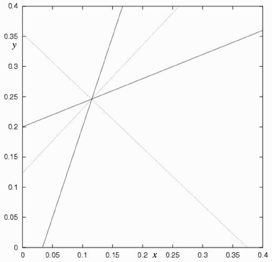
\(\text{FIGURE II.3}\)

Given the Equations to three straight lines, can we find the area of the triangle bounded by them? To find a general algebraic expression might be a bit tedious, though the reader might like to try it, but a numerical example is straightforward. For example, consider the lines

\[x - 5y + 12 = 0, \label{2.2.25} \tag{2.2.25}\]

\[3x + 4y - 9 = 0, \label{2.2.26} \tag{2.2.26}\]

\[3x - y - 3 = 0. \label{2.2.27} \tag{2.2.27}\]

By solving the Equations in pairs, it is soon found that they intersect at the points (−0.15789, 2.36842), (1.4, 1.2) and (1.92857, 2.78571). Application of Equation \(\ref{2.2.12}\) then gives the area as 1.544. The triangle is drawn in figure \(\text{II.4}\). Measure any side and the corresponding height with a ruler and see if the area is indeed about 1.54.

But now consider the three lines

\[x - 5y + 12 = 0, \label{2.2.28} \tag{2.2.28}\]

\[3x + 4y - 9 = 0 , \label{2.2.29} \tag{2.2.29}\]

\[3x + 23y - 54 = 0. \label{2.2.30} \tag{2.2.30}\]

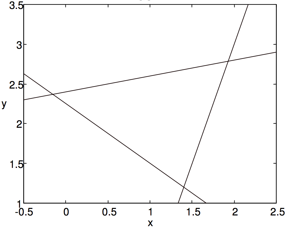
\(\text{FIGURE II.4}\)

By solving the Equations in pairs, it will be found that all three lines intersect at the same point (please do this), and the area of the triangle is, of course, zero. Any one of these Equations is, in fact, a linear combination of the other two. You should draw these three lines accurately on graph paper (or by computer). In general, if three lines are

\[A_1 x + B_1 y + C_1 = 0 \label{2.2.31} \tag{2.2.31}\]

\[A_2 x + B_2y + C_2 = 0 \label{2.2.32} \tag{2.2.32}\]

\[A_3 x + B_3 y + C_3 = 0 \label{2.2.33} \tag{2.2.33}\]

they will be concurrent at a single point if

\begin{array}{| c c c | c}
A_1 & B_1 & C_1 \\
A_2 & B_2 & C_2 & = 0. \\
A_3 & B_3 & C_3 \\
\label{2.2.34} \tag{2.2.34}
\end{array}

Thus the determinant in Equation \(\ref{2.2.12}\) provides a test of whether three points are collinear, and the determinant in Equation \(\ref{2.2.34}\) provides a test of whether three lines are concurrent.

Finally - at least for the present chapter - there may be rare occasion to write the Equation of a straight line in polar coordinates. It should be evident from figure \(\text{II.5}\) that the Equations

\[r = p \csc (\theta - \alpha) \ \text{or} \ r = p \csc (\alpha - \theta) \label{2.2.35} \tag{2.2.35}\]

describe a straight line passing at a distance \(p\) from the pole and making an angle \(\alpha\) with the initial line. If \(p = 0\), the polar Equation is merely \(\theta = \alpha\).

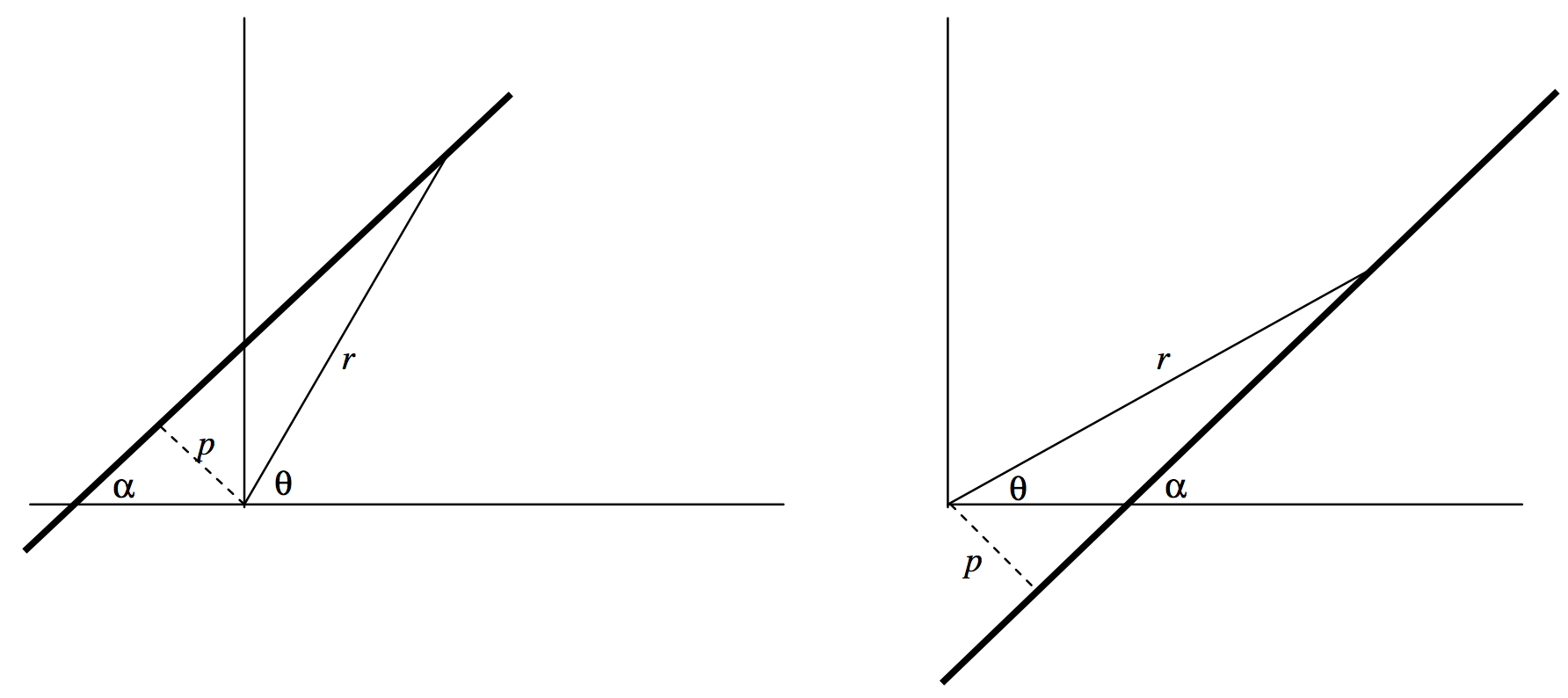
\(\text{FIGURE II.5}\)