2.4: The Hyperbola
- Page ID
- 6795
\( \newcommand{\vecs}[1]{\overset { \scriptstyle \rightharpoonup} {\mathbf{#1}} } \)
\( \newcommand{\vecd}[1]{\overset{-\!-\!\rightharpoonup}{\vphantom{a}\smash {#1}}} \)
\( \newcommand{\dsum}{\displaystyle\sum\limits} \)
\( \newcommand{\dint}{\displaystyle\int\limits} \)
\( \newcommand{\dlim}{\displaystyle\lim\limits} \)
\( \newcommand{\id}{\mathrm{id}}\) \( \newcommand{\Span}{\mathrm{span}}\)
( \newcommand{\kernel}{\mathrm{null}\,}\) \( \newcommand{\range}{\mathrm{range}\,}\)
\( \newcommand{\RealPart}{\mathrm{Re}}\) \( \newcommand{\ImaginaryPart}{\mathrm{Im}}\)
\( \newcommand{\Argument}{\mathrm{Arg}}\) \( \newcommand{\norm}[1]{\| #1 \|}\)
\( \newcommand{\inner}[2]{\langle #1, #2 \rangle}\)
\( \newcommand{\Span}{\mathrm{span}}\)
\( \newcommand{\id}{\mathrm{id}}\)
\( \newcommand{\Span}{\mathrm{span}}\)
\( \newcommand{\kernel}{\mathrm{null}\,}\)
\( \newcommand{\range}{\mathrm{range}\,}\)
\( \newcommand{\RealPart}{\mathrm{Re}}\)
\( \newcommand{\ImaginaryPart}{\mathrm{Im}}\)
\( \newcommand{\Argument}{\mathrm{Arg}}\)
\( \newcommand{\norm}[1]{\| #1 \|}\)
\( \newcommand{\inner}[2]{\langle #1, #2 \rangle}\)
\( \newcommand{\Span}{\mathrm{span}}\) \( \newcommand{\AA}{\unicode[.8,0]{x212B}}\)
\( \newcommand{\vectorA}[1]{\vec{#1}} % arrow\)
\( \newcommand{\vectorAt}[1]{\vec{\text{#1}}} % arrow\)
\( \newcommand{\vectorB}[1]{\overset { \scriptstyle \rightharpoonup} {\mathbf{#1}} } \)
\( \newcommand{\vectorC}[1]{\textbf{#1}} \)
\( \newcommand{\vectorD}[1]{\overrightarrow{#1}} \)
\( \newcommand{\vectorDt}[1]{\overrightarrow{\text{#1}}} \)
\( \newcommand{\vectE}[1]{\overset{-\!-\!\rightharpoonup}{\vphantom{a}\smash{\mathbf {#1}}}} \)
\( \newcommand{\vecs}[1]{\overset { \scriptstyle \rightharpoonup} {\mathbf{#1}} } \)
\(\newcommand{\longvect}{\overrightarrow}\)
\( \newcommand{\vecd}[1]{\overset{-\!-\!\rightharpoonup}{\vphantom{a}\smash {#1}}} \)
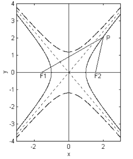
\(\newcommand{\avec}{\mathbf a}\) \(\newcommand{\bvec}{\mathbf b}\) \(\newcommand{\cvec}{\mathbf c}\) \(\newcommand{\dvec}{\mathbf d}\) \(\newcommand{\dtil}{\widetilde{\mathbf d}}\) \(\newcommand{\evec}{\mathbf e}\) \(\newcommand{\fvec}{\mathbf f}\) \(\newcommand{\nvec}{\mathbf n}\) \(\newcommand{\pvec}{\mathbf p}\) \(\newcommand{\qvec}{\mathbf q}\) \(\newcommand{\svec}{\mathbf s}\) \(\newcommand{\tvec}{\mathbf t}\) \(\newcommand{\uvec}{\mathbf u}\) \(\newcommand{\vvec}{\mathbf v}\) \(\newcommand{\wvec}{\mathbf w}\) \(\newcommand{\xvec}{\mathbf x}\) \(\newcommand{\yvec}{\mathbf y}\) \(\newcommand{\zvec}{\mathbf z}\) \(\newcommand{\rvec}{\mathbf r}\) \(\newcommand{\mvec}{\mathbf m}\) \(\newcommand{\zerovec}{\mathbf 0}\) \(\newcommand{\onevec}{\mathbf 1}\) \(\newcommand{\real}{\mathbb R}\) \(\newcommand{\twovec}[2]{\left[\begin{array}{r}#1 \\ #2 \end{array}\right]}\) \(\newcommand{\ctwovec}[2]{\left[\begin{array}{c}#1 \\ #2 \end{array}\right]}\) \(\newcommand{\threevec}[3]{\left[\begin{array}{r}#1 \\ #2 \\ #3 \end{array}\right]}\) \(\newcommand{\cthreevec}[3]{\left[\begin{array}{c}#1 \\ #2 \\ #3 \end{array}\right]}\) \(\newcommand{\fourvec}[4]{\left[\begin{array}{r}#1 \\ #2 \\ #3 \\ #4 \end{array}\right]}\) \(\newcommand{\cfourvec}[4]{\left[\begin{array}{c}#1 \\ #2 \\ #3 \\ #4 \end{array}\right]}\) \(\newcommand{\fivevec}[5]{\left[\begin{array}{r}#1 \\ #2 \\ #3 \\ #4 \\ #5 \\ \end{array}\right]}\) \(\newcommand{\cfivevec}[5]{\left[\begin{array}{c}#1 \\ #2 \\ #3 \\ #4 \\ #5 \\ \end{array}\right]}\) \(\newcommand{\mattwo}[4]{\left[\begin{array}{rr}#1 \amp #2 \\ #3 \amp #4 \\ \end{array}\right]}\) \(\newcommand{\laspan}[1]{\text{Span}\{#1\}}\) \(\newcommand{\bcal}{\cal B}\) \(\newcommand{\ccal}{\cal C}\) \(\newcommand{\scal}{\cal S}\) \(\newcommand{\wcal}{\cal W}\) \(\newcommand{\ecal}{\cal E}\) \(\newcommand{\coords}[2]{\left\{#1\right\}_{#2}}\) \(\newcommand{\gray}[1]{\color{gray}{#1}}\) \(\newcommand{\lgray}[1]{\color{lightgray}{#1}}\) \(\newcommand{\rank}{\operatorname{rank}}\) \(\newcommand{\row}{\text{Row}}\) \(\newcommand{\col}{\text{Col}}\) \(\renewcommand{\row}{\text{Row}}\) \(\newcommand{\nul}{\text{Nul}}\) \(\newcommand{\var}{\text{Var}}\) \(\newcommand{\corr}{\text{corr}}\) \(\newcommand{\len}[1]{\left|#1\right|}\) \(\newcommand{\bbar}{\overline{\bvec}}\) \(\newcommand{\bhat}{\widehat{\bvec}}\) \(\newcommand{\bperp}{\bvec^\perp}\) \(\newcommand{\xhat}{\widehat{\xvec}}\) \(\newcommand{\vhat}{\widehat{\vvec}}\) \(\newcommand{\uhat}{\widehat{\uvec}}\) \(\newcommand{\what}{\widehat{\wvec}}\) \(\newcommand{\Sighat}{\widehat{\Sigma}}\) \(\newcommand{\lt}{<}\) \(\newcommand{\gt}{>}\) \(\newcommand{\amp}{&}\) \(\definecolor{fillinmathshade}{gray}{0.9}\)A hyperbola is the locus of a point that moves such that the difference between its distances from two fixed points called the foci is constant. We shall call the difference between these two distances \(2a\) and the distance between the foci \(2ae\), where \(e\) is the eccentricity of the hyperbola, and is a number greater than 1. See figure \(\text{II.28}\).
\(\text{FIGURE II.28}\)
For example, in a Young's double-slit interference experiment, the \(m\)th bright fringe is located at a point on the screen such that the path difference for the rays from the two slits is \(m\) wavelengths. As the screen is moved forward or backwards, this relation continues to hold for the \(m\)th bright fringe, whose locus between the slits and the screen is therefore a hyperbola. The "Decca" system of radar navigation, first used at the D-Day landings in the Second World War and decommissioned only as late as 2000 on account of being rendered obsolete by the "GPS" (Global Positioning Satellite) system, depended on this property of the hyperbola. (Since writing this, part of the Decca system has been re-commissioned as a back-up in case of problems with GPS.) Two radar transmitters some distance apart would simultaneously transmit radar pulses. A ship would receive the two signals separated by a short time interval, depending on the difference between the distances from the ship to the two transmitters. This placed the ship on a particular hyperbola. The ship would also listen in to another pair of transmitters, and this would place the ship on a second hyperbola. This then placed the ship at one of the four points where the two hyperbolas intersected. It would usually be obvious which of the four points was the correct one, but any ambiguity could be resolved by the signals from a third pair of transmitters.
In figure \(\text{II.28}\), the coordinates of \(F_1\) and \(F_2\) are, respectively, \((−ae , 0)\) and \((ae , 0)\).
The condition \(\text{PF}_1 − \text{PF}_2 = 2a\) requires that
\[\left[ (x + ae)^2 + y^2 \right]^{\dfrac{1}{2}} - \left[ (x-ae)^2 + y^2 \right]^{\dfrac{1}{2}} = 2a, \label{2.5.1} \tag{2.5.1}\]
and this is the Equation to the hyperbola. After some arrangement, this can be written
\[\dfrac{x^2}{a^2} - \dfrac{y^2}{a^2 (e^2 -1)} = 1, \label{2.5.2} \tag{2.5.2}\]
which is a more familiar form for the Equation to the hyperbola. Let us define a length \(b\) by
\[b^2 = a^2 (e^2 - 1). \label{2.5.3} \tag{2.5.3}\]
The Equation then becomes
\[\dfrac{x^2}{a^2} - \dfrac{y^2}{b^2} = 1, \label{2.5.4} \tag{2.5.4}\]
which is the most familiar form for the Equation to a hyperbola.
When a meteor streaks across the sky, it can be tracked by radar. The radar instrumentation can determine the range (distance) of the meteoroid as a function of time. Show that, if the meteoroid is moving at constant speed (a questionable assumption, because it must be decelerating, but perhaps we can assume the decrease in speed is negligible during the course of the observation), and if the range \(r\) is plotted against the time, the graph will be a hyperbola. Show also that, if \(r^2\) is plotted against \(t\), the graph will be a parabola of the form
\[r^2 = a t^2 + bt + c, \]
where \(a=V^2 , \ b = -2V^2 t_0, \ c = V^2 t_0^2 + r_0^2, \ V = \text{speed of the meteoroid}, \ t_0 = \text{time of closest approach}, \ r_0 = \text{distance of closest approach}\).
Radar observation of a meteor yields the following range-time data:
\begin{array}{c l}
t(\text{s}) & r(\text{km}) \\
\\
0.0 & 101.4 \ *\\
0.1 & 103.0 \\
0.2 & 105.8 \\
0.3 & 107.8 \\
0.4 & 111.1 \\
0.5 & 112.6 \\
0.6 & 116.7 \\
0.7 & 119.3 \\
0.8 & 123.8 \ * \\
0.9 & 126.4 \\
1.0 & 130.6 \\
1.1 & 133.3 \\
1.2 & 138.1 \\
1.3 & 141.3 \ * \\
\end{array}
Assume that the velocity of the meteor is constant.
Determine i. The time of closest approach (to 0.01 \(\text{s}\))
ii. The distance of closest approach (to 0.1 \(\text{km}\))
iii. The speed (to 1.0 \(\text{km s}^{-1}\))
If you wish, just use the three asterisked data to determine \(a\), \(b\) and \(c\). If you are more energetic, use all the data, and determine \(a\), \(b\) and \(c\) by least squares, and the probable errors of \(V\), \(t_0\) and \(r_0\).
The distance between the two vertices of the hyperbola is its transverse axis, and the length of the semi transverse axis is \(a\) − but what is the geometric meaning of the length \(b\)? This is discussed below in the next subsection (on the conjugate hyperbola) and again in a later section on the impact parameter.
The lines perpendicular to the \(x\)-axis and passing through the foci are the two latera recta. Since the foci are at \((\pm ae , \ 0)\), the points where the latera recta intersect the hyperbola can be found by putting \(x = ae\) into the Equation to the hyperbola, and it is then found that the length \(l\) of a semi latus rectum is
\[l = a(e^2 -1 ) . \label{2.5.5} \tag{2.5.5}\]
The Equation
\[\dfrac{x^2}{a^2} - \dfrac{y^2}{b^2} = -1 \label{2.5.6} \tag{2.5.6}\]
is the Equation to the conjugate hyperbola.
The conjugate hyperbola is drawn dashed in figure \(\text{II.28}\), and it is seen that the geometric meaning of \(b\) is that it is the length of the semi transverse axis of the conjugate hyperbola. It is a simple matter to show that the eccentricity of the conjugate hyperbola is \(e/\sqrt{e^2-1}\).
The lines \[y = \pm \dfrac{bx}{a} \label{2.5.7} \tag{2.5.7}\]
are the asymptotes of the hyperbola.
Equation \ref{2.5.7} can also be written
\[\dfrac{x^2}{a^2} - \dfrac{y^2}{b^2} = 0. \label{2.5.8} \tag{2.5.8}\]
Thus
\[ \dfrac{x^2}{a^2} - \dfrac{y^2}{b^2} = c \label{2.5.9} \tag{2.5.9}\]
is the hyperbola, the asymptotes, or the conjugate hyperbola, if \(c = +1\), \(0\) or \(−1\) respectively. The asymptotes are drawn as dotted lines in figure \(\text{II.28}\).
The semi angle ψ between the asymptotes is given by
\[\tan ψ = b/a. \label{2.5.10} \tag{2.5.10}\]
If the eccentricity of a hyperbola is \(e\), show that the eccentricity of its conjugate is \(\dfrac{e}{\sqrt{e^2 - 1}}\).
No one will be surprised to note that this implies that, if the eccentricities of a hyperbola and its conjugate are equal, then each is equal to \(\sqrt{2}\).
The Directrices
The lines \(y = \pm a / e\) are the directrices, and, as with the ellipse (and with a similar proof), the hyperbola has the property that the ratio of the distance \(\text{PF}_2\) to a focus to the distance \(\text{PN}\) to the directrix is constant and is equal to the eccentricity of the hyperbola. This ratio (i.e. the eccentricity) is less than one for the ellipse, equal to one for the parabola, and greater than one for the hyperbola. It is not a property that will be of great importance for our purposes, but is worth mentioning because it is a property that is sometimes used to define a hyperbola. I leave it to the reader to draw the directrices in their correct positions in figure \(\text{II.28}\).
Parametric Equations to the Hyperbola.
The reader will recall that the point \((a \cos E, b \sin E)\) is on the ellipse \((x^2/a^2) + \left( y^2/b^2 \right) = 1\) and that this is evident because this Equation is the \(E\)-eliminant of \(x = a \cos E\) and \(y = b \sin E\). The angle \(E\) has a geometric interpretation as the eccentric anomaly. Likewise, recalling the relation \(\cosh^2 \phi − \sinh^2 \phi = 1\), it will be evident that \((x^2 / a^2) - \left(y^2/b^2 \right) = 1\) can also be obtained as the \(\phi\)−eliminant of the Equations
\[x = a \cosh \phi, \quad y = b \sinh \phi \label{2.5.11} \tag{2.5.11}\]
These two Equations are therefore the parametric Equations to the hyperbola, and any point satisfying these two Equations lies on the hyperbola. The variable \(\phi\) is not an angle, and has no geometric interpretation analogous to the eccentric anomaly of an ellipse. The Equations
\[x = a \sec E, \quad y = b \tan E \label{2.5.12} \tag{2.5.12}\]
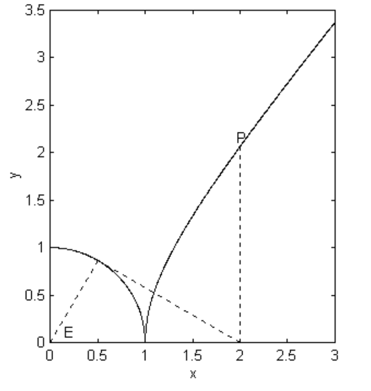
can also be used as parametric Equations to the hyperbola, on account of the trigonometric identity \(1 + \tan^2 E = \sec^2 E\). In that case, the angle \(E\) does have a geometric interpretation (albeit not a particularly interesting one) in relation to the auxiliary circle, which is the circle of radius a centred at the origin. The meaning of the angle should be evident from figure \(\text{II.29}\), in which \(E\) is the eccentric angle corresponding to the point \(\text{P}\).
\(\text{FIGURE II.29}\)
Impact Parameter
A particle travelling very fast under the action of an inverse square attractive force (such as an interstellar meteoroid or comet - if there are such things - passing by the Sun, or an electron in the vicinity of a positively charged atomic nucleus) will move in a hyperbolic path. We prove this in a later chapter, as well as discussing the necessary speed. We may imagine the particle initially approaching from a great distance along the asymptote at the bottom right hand corner of figure \(\text{II.30}\). As it approaches the focus, it no longer moves along the asymptote but along an arm of the hyperbola.
\(\text{FIGURE II.30}\)
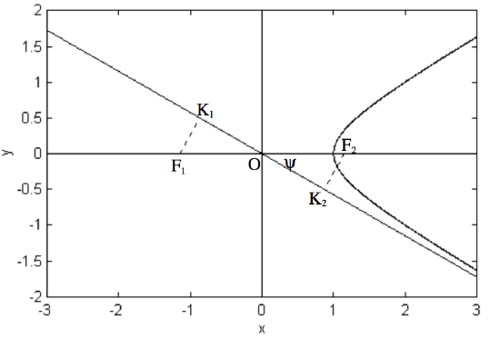
The distance \(\text{K}_2 \ \text{F}_2\), which is the distance by which the particle would have missed \(\text{F}_2\) in the absence of an attractive force, is commonly called the impact parameter. Likewise, if the force had been a repulsive force (for example, suppose the moving particle were a positively charged particle and there were a centre of repulsion at \(\text{F}_1\), \(\text{F}_1\text{K}_1\) would be the impact parameter. Clearly, \(\text{F}_1\text{K}_1\) and \(\text{F}_2\text{K}_2\) are equal in length. The symbol that is often used in scattering theory, whether in celestial mechanics or in particle physics, is \(b\) - but is this \(b\) the same \(b\) that goes into the Equation to the hyperbola and which is equal to the semi major axis of the conjugate hyperbola?
\(\text{OF}_2 = ae\), and therefore \(\text{K}_2\text{F}_2 = ae \sin ψ\). This, in conjunction with \(\tan ψ = b/a\) and \(b^2 = a^2 (e^2 − 1)\), will soon show that the impact parameter is indeed the same \(b\) that we are familiar with, and that \(b\) is therefore a very suitable symbol to use for impact parameter.
Tangents to the Hyperbola
Using the same arguments as for the ellipse, the reader should easily find that lines of the form
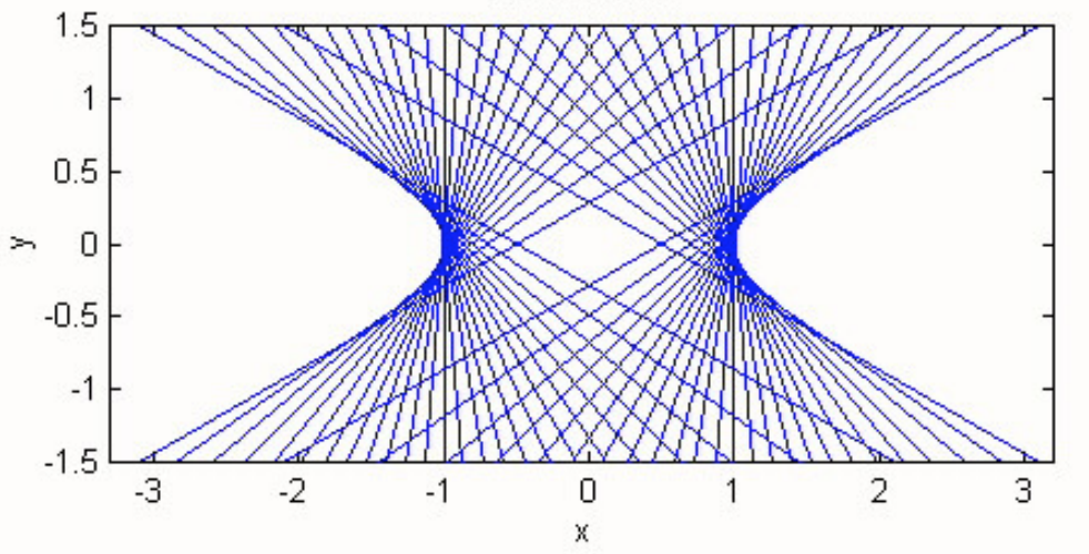
\[y = mx \pm \sqrt{a^2 m^2 - b^2} \tag{2.5.13} \label{2.5.13}\]
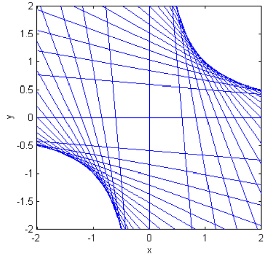
are tangent to the hyperbola. This is illustrated in figure \(\text{II.33}\) for a hyperbola with \(b = a /2\), with tangents drawn with slopes \(30^\circ\) to \(150^\circ\) in steps of \(5^\circ\). (The asymptotes have \(ψ = 26^\circ 34^\prime\).) (Sorry, but there are no figures \(\text{II.31}\) or \(\text{II.32}\) - computer problems!)
\(\text{FIGURE II.31}\)
Likewise, from similar arguments used for the ellipse, the tangent to the hyperbola at the point \((x ,y)\) is found to be
\[\frac{x_1x}{a^2} - \dfrac{y_1y}{b^2} = 1. \label{2.5.14} \tag{2.5.14}\]
Director Circle
As for the ellipse, and with a similar derivation, the locus of the points of intersection of perpendicular tangents is a circle, called the director circle, which is of radius \(√(a^2 − b^2 )\). This is not of particular importance for our purposes, but the reader who is interested might like to prove this by the same method as was done for the director circle of the ellipse, and might like to try drawing the circle and some tangents. If \(b > a\), that is to say if \(ψ > 45^\circ\) and the angle between the asymptotes is greater than \(90^\circ\), the director circle is not real and it is of course not possible to draw perpendicular tangents.
Rectangular Hyperbola
If the angle between the asymptotes is \(90^\circ\), the hyperbola is called a rectangular hyperbola. For such a hyperbola, \(b = a\), the eccentricity is \(√2\), the director circle is a point, namely the origin, and perpendicular tangents can be drawn only from the asymptotes.
The Equation to a rectangular hyperbola is
\[x^2 - y^2 = a^2 \label{2.5.15} \tag{2.5.15}\]
and the asymptotes are at \(45^\circ\) to the \(x\) axis.
Let \(\text{O}x^\prime, \ \text{O}y^\prime\) be a set of axes at \(45^\circ\) to the \(x\) axis. (That is to say, they are the asymptotes of the rectangular hyperbola.) Then the Equation to the rectangular hyperbola referred to its asymptotes as coordinate axes is found by the substitutions
\[\pmatrix{x \\ y} = \pmatrix{\cos 45^\circ & \sin 45^\circ \\ - \sin 45^\circ & \cos 45^\circ} \pmatrix{x^\prime \\ y^\prime} \tag{2.5.16} \label{2.5.16}\]
into \(x^2 − y^2 = a^2\). This results in the Equation
\[x^\prime y^\prime = \frac{1}{2} a^2 = c^2 , \quad \text{where} \quad c= a/\sqrt{2}, \label{2.5.17} \tag{2.5.17}\]
for the Equation to the rectangular hyperbola referred to its asymptotes as coordinate axes. The geometric interpretation of \(c\) is shown in figure \(\text{II.32}\), which is drawn for \(c = 1\), and we have called the coordinate axes \(x\) and \(y\). The length of the semi transverse axis is \(c \sqrt{2}\).
\(\text{FIGURE II.32}\)
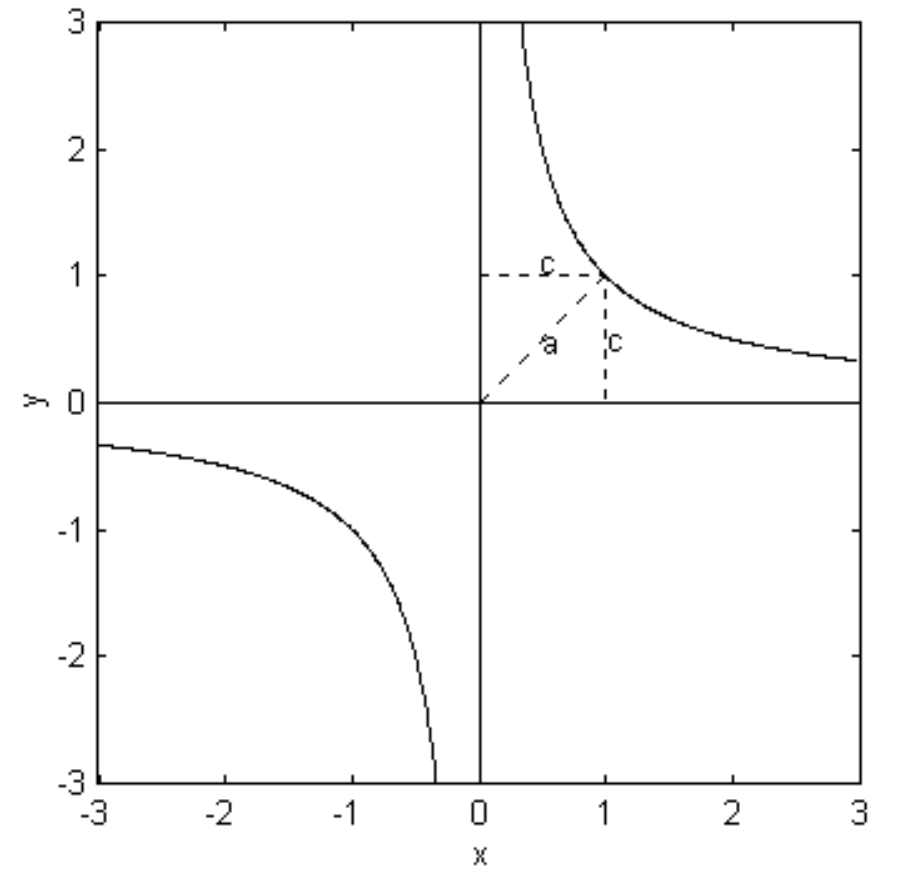
The simple Equation \(y = 1/x\) is a rectangular hyperbola and indeed it is this Equation that is shown in figure \(\text{II.32}\).
It is left to the reader to show that the parametric Equations to the rectangular hyperbola \(xy = c^2\) (we have dropped the primes) are \(x = ct, \ y = c/t\), that lines of the form \(y=mx \pm 2c \sqrt{-m}\) are tangent to \(xy = c^2\) (figure II.35, drawn with slopes from \(90^\circ\) to \(180^\circ\) in steps of \(5^\circ\) ), and that the tangent at \((x_1 , y_1 )\) is \(x_1y + y_1x = 2c\).
\(\text{FIGURE II.33}\)
Equation of a Hyperbola Referred to its Asymptotes as Axes of Coordinates
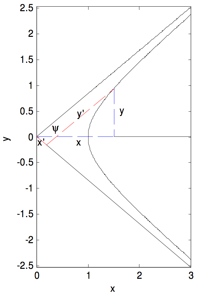
We have shown that the Equation to a rectangular hyperbola referred to its asymptotes as axes of coordinates is \(x^\prime y^\prime = \frac{1}{2} a^2 = c^2\). In fact the Equation \(x^\prime y^\prime = c^2\) is the Equation to any hyperbola (centred at \((0 ,\ 0)\)), not necessarily rectangular, when referred to its asymptotes as axes of coordinates, where \(c^2 = \frac{1}{4} (a^2 + b^2)\) In the figure below I have drawn a hyperbola and a point on the hyperbola whose coordinates with respect to the horizontal and vertical axes are \((x , \ y)\), and whose coordinates with respect to the asymptotes are \((x^\prime , y^\prime)\). I have shown the distances \(x\) and \(y\) with blue dashed lines, and the distances \(x^\prime\) and \(y^\prime\) with red dashed lines. The semiangle between the asymptotes is \(ψ\).
The Equation to the hyperbola referred to the horizontal and vertical axes is
\[\frac{x^2}{a^2} - \frac{y^2}{b^2} = 1. \label{2.5.18} \tag{2.5.18}\]
From the drawing, we see that
\[x = (x^\prime + y^\prime) \cos ψ, \quad y = (y^\prime - x^\prime) \sin ψ. \label{2.5.19a,b} \tag{2.5.19a,b}\]
If we substitute these into Equation \(\ref{2.5.18}\), and also make use of the relation \(\tan ψ = b/a\) (Equation \(\ref{2.5.10}\)), we arrive at the Equation to the hyperbola referred to the asymptotes as axes of coordinates:
\[x^\prime y^\prime = \frac{1}{4}(a^2 + b^2) = c^2 . \label{2.5.20} \tag{2.5.20}\]
Polar Equation to the Hyperbola
We found the polar Equations to the ellipse and the parabola in different ways. Now go back and look at both methods and use either (or both) to show that the polar Equation to the hyperbola (focus as pole) is
\[r = \frac{l}{1+ e \cos \theta}. \tag{2.5.21} \label{2.5.21}\]
This is the polar Equation to any conic section - which one being determined solely by the value of \(e\). You should also ask yourself what is represented by the Equation
\[r = \frac{l}{1-e \cos \theta}. \label{2.5.22} \tag{2.5.22}\]
Try sketching it for different values of \(e\).


