2.3: The Parabola

We define a parabola as the locus of a point that moves such that its distance from a fixed straight line called the directrix is equal to its distance from a fixed point called the focus. Unlike the ellipse, a parabola has only one focus and one directrix. However, comparison of this definition with the focus - directrix property of the ellipse (which can also be used to define the ellipse) shows that the parabola can be regarded as a limiting form of an ellipse with eccentricity equal to unity.

We shall find the Equation to a parabola whose directrix is the line \(y = −q\) and whose focus is the point \((q , 0)\). Figure \(\text{II.20}\) shows the parabola. \(\text{F}\) is the focus and \(\text{O}\) is the origin of the coordinate system. The vertex of the parabola is at the origin. In an orbital context, for example, the orbit of a comet moving around the Sun in parabolic orbit, the Sun would be at the focus \(\text{F}\), and the distance between vertex and focus would be the perihelion distance, for which the symbol \(q\) is traditionally used in orbit theory.

\(\text{FIGURE II.20}\)

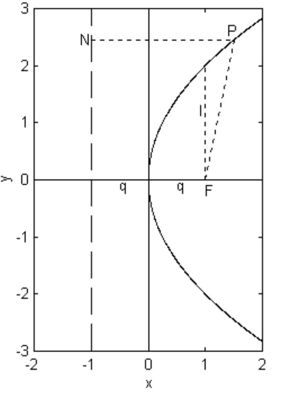
From figure \(\text{II.20}\), it is evident that the definition of the parabola \((\text{PF} = \text{PN})\) requires that

\[(x-q)^2 + y^2 = (x+q)^2 , \label{2.4.1} \]

from which

\[y^2 = 4qx , \label{2.4.2}\]

which is the Equation to the parabola.

Exercise \(\PageIndex{1}\)

Sketch the following parabolas:

1. \(y^2 = -4qx \)
2. \(x^2 = 4qy\)
3. \(x^2 = -4qy,\)
4. \((y-2)^2 = 4q (x-3).\)

The line parallel to the \(y\)-axis and passing through the focus is the latus rectum. Substitution of \(x = q\) into \(y^2 = 4ax\) shows that the latus rectum intersects the parabola at the two points \((q , \pm 2q)\), and that the length \(l\) of the semi latus rectum is \(2q\).

The Equations

\[x = qt^2 , \quad y = 2qt \label{2.4.3} \]

are the parametric Equations to the parabola, for \(y^2 = 4qx\) results from the elimination of \(t\) between them. In other words, if \(t\) is any variable, then any point that satisfies these two Equations lies on the parabola.

Most readers will know that if a particle is moving with constant speed in one direction and constant acceleration at right angles to that direction, as with a ball projected in a uniform gravitational field or an electron moving in a uniform electric field, the path is a parabola. In the constant speed direction the distance is proportional to the time, and in the constant acceleration direction, the distance is proportional to the square of the time, and hence the path is a parabola.

Tangents to a Parabola.

Where does the straight line \(y = mx + c\) intersect the parabola \(y^2 = 4qx\)? The answer is found by substituting \(mx + c\) for \(y\) to obtain, after rearrangement,

\[m^2 x^2 + 2(mc - 2q) x + c^2 = 0 . \label{2.4.4} \]

The line is tangent if the discriminant is zero, which leads to

\[c = q/m . \label{2.4.5} \]

Thus a straight line of the form

\[y = mx + q/m \label{2.4.6} \]

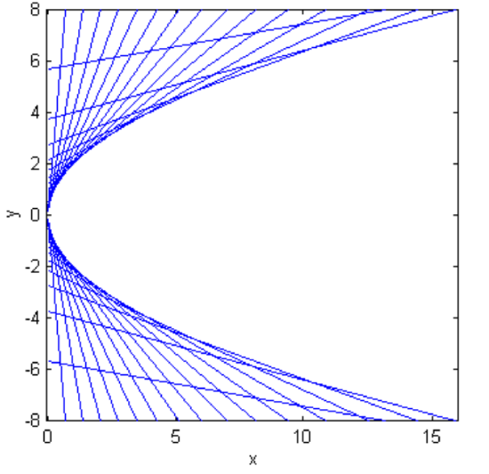
is tangent to the parabola. Figure \(\text{II.22}\) illustrates this for several lines, the slopes of each differing by \(5^\circ\) from the next.

\(\text{FIGURE II.22}\)

We shall now derive an Equation to the line that is tangent to the parabola at the point \((x_1 , y_1 )\).

Let \((x_1 , y_1) = (qt_1^2 , 2qt_1)\) be a point on the parabola, and
Let \((x_2 , y_2) = (qt_2^2 , 2qt_2)\) be another point on the parabola.

The line joining these two points is

\[\frac{y-2qt_1}{x-qt_1^2} = \frac{2q(t_2 - t_1)}{q(t_2^2 - t_1^2)} = \frac{2}{t_2+t_1}. \label{2.4.7} \]

Now let \(t_2\) approach \(t_1\), eventually coinciding with it. Putting \(t_1 = t_2 = t\) in the last Equation results, after simplification, in

\[ty = x + qt^2 , \label{2.4.8} \]

being the Equation to the tangent at \((qt^2 , 2qt )\).

Multiply by \(2q\):

\[2qty = 2q (x+qt^2) \label{2.4.9} \]

and it is seen that the Equation to the tangent at \((x_1 , y_1 )\) is

\[y_1 y = 2q (x_1 + x). \label{2.4.10} \]

There are a number of interesting geometric properties, some of which are given here. For example, if a tangent to the parabola at a point \(P\) meets the directrix at \(Q\), then, just as for the ellipse, \(P\) and \(Q\) subtend a right angle at the focus (figure \(\text{II.23}\)). The proof is similar to that given for the ellipse, and is left for the reader.

\(\text{FIGURE II.23}\)

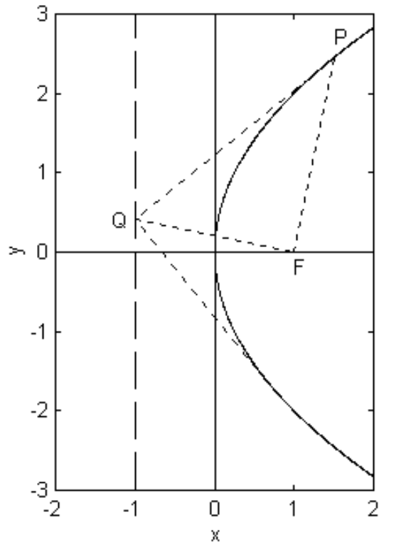
The reader will recall that perpendicular tangents to an ellipse meet on the director circle. The analogous theorem vis-à-vis the parabola is that perpendicular tangents meet on the directrix. This is also illustrated in figure \(\text{II.23}\). The theorem is not specially important in orbit theory, and the proof is also left to the reader.

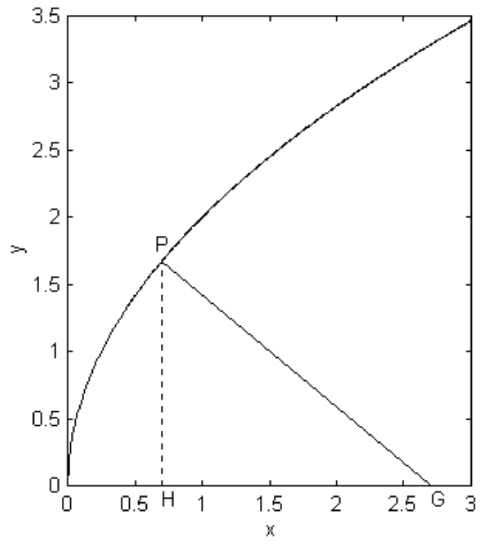
Let \(\text{PG}\) be the normal to the parabola at point \(\text{P}\), meeting the axis at \(\text{G}\) (figure \(\text{II.24}\)). We shall call the length \(\text{GH}\) the subnormal. A curious property is that the length of \(\text{GH}\) is always equal to \(l\), the length of the semi latus rectum (which in figure \(\text{II.24}\) is of length 2 − i.e. the ordinate where \(x = 1\)), irrespective of the position of \(\text{P}\). This proof again is left to the reader.

\(\text{FIGURE II.24}\)

The following two geometrical properties, while not having immediate applications to orbit theory, certainly have applications to astronomy.

\(\text{FIGURE II.25}\)

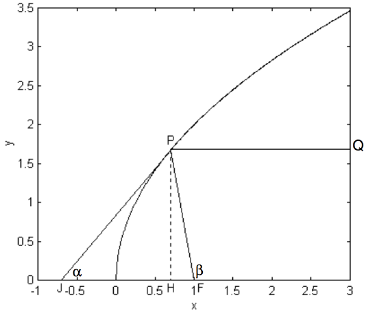
The tangent at \(\text{P}\) makes an angle \(\alpha\) with the \(x\)-axis, and \(\text{PF}\) makes an angle \(\beta\) with the \(x\)-axis (figure \(\text{II.25}\)). We shall show that \(\beta = 2\alpha\) and deduce an interesting consequence.

The Equation to the tangent (see Equation \(\ref{2.4.8}\)) is \(ty = x + qt^2\), which shows that

\[\tan \alpha = 1/t . \label{2.4.11} \]

The coordinates of \(\text{P}\) and \(\text{F}\) are, respectively, \(\left(qt^2 , 2qt \right)\) and \((q , 0)\), and so, from the triangle \(\text{PFH}\), we find.

\[\tan \beta = \frac{2t}{t^2-1}. \label{2.4.12}\]

Let \(\tau = 1/t\), then \(\tan \alpha = \tau\) and \(\tan \beta = 2\tau/(1 - \tau^2)\), which shows that \(\beta = 2\alpha\).

This also shows that triangle \(\text{JFP}\) is isosceles, with the angles at \(\text{J}\) and \(\text{P}\) each being \(\alpha\). This can also be shown as follows.

From the Equation \(ty = x + qt^2\), we see that \(\text{J}\) is the point \((−qt^2 , 0)\), so that \(\text{JF} = q (t^2 + 1)\).

From triangle \(\text{PFH}\), we see that

\[(\text{PF})^2 = 4q^2 t^2 + q^2 \left(t^2 - 1 \right)^2 - q^2 \left( t^2 + 1 \right)^2 . \label{2.4.13}\]

Therefore \[\text{PF} = \text{JF} . \label{2.4.14}\]

Either way, since the triangle \(\text{JPF}\) is isosceles, it follows that \(\text{QP}\) and \(\text{PF}\) make the same angle \(\alpha\) to the tangent. If the parabola is a cross section of a telescopic mirror, any ray of light coming in parallel to the axis will be focussed at \(\text{F}\), so that a paraboloidal mirror, used on-axis, does not suffer from spherical aberration. (This property holds, of course, only for light parallel to the axis of the paraboloid, so that a paraboloidal mirror, without some sort of correction, gives good images over only a narrow field of view.)

Now consider what happens when you stir a cup of tea. The surface takes up a shape that looks as though it might resemble the parabola \(y = x^2 /(4q)\) - see figure \(\text{II.26}\):

\(\text{FIGURE II.26}\)

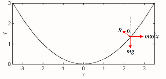
Suppose the liquid is circulating at angular speed \(ω\). A tea leaf floating on the surface is in equilibrium (in the rotating reference frame) under three forces: its weight \(mg\), the centrifugal force \(mω^2 x\) and the normal reaction \(R\). The normal to the surface makes an angle \(\theta\) with the vertical (and the tangent makes an angle \(\theta\) with the horizontal) given by

\[\tan \theta = \frac{ω^2x}{g}. \label{2.4.15} \]

But the slope of the parabola \(y = x^2 /(4q)\) is \(x/(2q)\), so that the surface is indeed a parabola with semi latus rectum \(2q = g/ω^2\).

This phenomenon has been used in Canada to make a successful large telescope (diameter \(6 \ \text{m}\) ) in which the mirror is a spinning disc of mercury that takes up a perfectly paraboloidal shape. Another example is the spin casting method that has been successfully used for the production of large, solid glass paraboloidal telescope mirrors. In this process, the furnace is rotated about a vertical axis while the molten glass cools and eventually solidifies into the required paraboloidal effect.

Exercise \(\PageIndex{1}\)

The 6.5 metre diameter mirrors for the twin Magellan telescopes at Las Campañas, Chile, have a focal ratio \(f/1.25\). They were made by the technique of spin casting at The University of Arizona's Mirror Laboratory. At what speed would the furnace have had to be rotated in order to achieve the desired focal ratio? (Answer \(= 7.4 \ \text{rpm}\).) Notice that \(f/1.25\) is quite a deep paraboloid. If this mirror had been made by traditional grinding from a solid disc, what volume of material would have had to be removed to make the desired paraboloid? (Answer - a whopping 5.4 cubic metres, or about 12 tons!)

Polar Equation to the Parabola

As with the ellipse, we choose the focus as pole and the axis of the parabola as initial line. We shall orient the parabola so that the vertex is toward the right, as in figure \(\text{II.27}\).

We recall the focus-directrix property, \(\text{FP} = \text{PN}\). Also, from the definition of the directrix, \(\text{FO}=\text{OM} = q\), so that \(\text{FM} = 2q = l\), the length of the semi latus rectum. It is therefore immediately evident from figure \(\text{II.27}\) that \(r \cos \theta + r = 2q = l\), so that the polar Equation to the parabola is

\[r = \frac{l}{1+ e ~\cos \theta}. \label{2.4.16} \]

\(\text{FIGURE II.27}\)

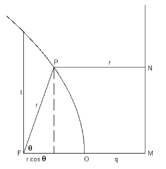
This is the same as the polar Equation to the ellipse (Equation 2.3.36), with \(e = 1\) for the parabola. I have given different derivations for the ellipse and for the parabola; the reader might like to interchange the two approaches and develop Equation 2.3.36 in the same manner as we have developed Equation \(\ref{2.4.16}\).

When we discuss the hyperbola, I shall ask you to show that its polar Equation is also the same as 2.3.36. In other words, Equation 2.3.36 is the Equation to a conic section, and it represents an ellipse, parabola or hyperbola according to whether \(e<1, \ e=1 \ \text{or } e>1\).