

13.2: Triangles
- Page ID
- 6869

\( \newcommand{\vecs}[1]{\overset { \scriptstyle \rightharpoonup} {\mathbf{#1}} } \)
\( \newcommand{\vecd}[1]{\overset{-\!-\!\rightharpoonup}{\vphantom{a}\smash {#1}}} \)
\( \newcommand{\dsum}{\displaystyle\sum\limits} \)
\( \newcommand{\dint}{\displaystyle\int\limits} \)
\( \newcommand{\dlim}{\displaystyle\lim\limits} \)
\( \newcommand{\id}{\mathrm{id}}\) \( \newcommand{\Span}{\mathrm{span}}\)
( \newcommand{\kernel}{\mathrm{null}\,}\) \( \newcommand{\range}{\mathrm{range}\,}\)
\( \newcommand{\RealPart}{\mathrm{Re}}\) \( \newcommand{\ImaginaryPart}{\mathrm{Im}}\)
\( \newcommand{\Argument}{\mathrm{Arg}}\) \( \newcommand{\norm}[1]{\| #1 \|}\)
\( \newcommand{\inner}[2]{\langle #1, #2 \rangle}\)
\( \newcommand{\Span}{\mathrm{span}}\)
\( \newcommand{\id}{\mathrm{id}}\)
\( \newcommand{\Span}{\mathrm{span}}\)
\( \newcommand{\kernel}{\mathrm{null}\,}\)
\( \newcommand{\range}{\mathrm{range}\,}\)
\( \newcommand{\RealPart}{\mathrm{Re}}\)
\( \newcommand{\ImaginaryPart}{\mathrm{Im}}\)
\( \newcommand{\Argument}{\mathrm{Arg}}\)
\( \newcommand{\norm}[1]{\| #1 \|}\)
\( \newcommand{\inner}[2]{\langle #1, #2 \rangle}\)
\( \newcommand{\Span}{\mathrm{span}}\) \( \newcommand{\AA}{\unicode[.8,0]{x212B}}\)
\( \newcommand{\vectorA}[1]{\vec{#1}} % arrow\)
\( \newcommand{\vectorAt}[1]{\vec{\text{#1}}} % arrow\)
\( \newcommand{\vectorB}[1]{\overset { \scriptstyle \rightharpoonup} {\mathbf{#1}} } \)
\( \newcommand{\vectorC}[1]{\textbf{#1}} \)
\( \newcommand{\vectorD}[1]{\overrightarrow{#1}} \)
\( \newcommand{\vectorDt}[1]{\overrightarrow{\text{#1}}} \)
\( \newcommand{\vectE}[1]{\overset{-\!-\!\rightharpoonup}{\vphantom{a}\smash{\mathbf {#1}}}} \)
\( \newcommand{\vecs}[1]{\overset { \scriptstyle \rightharpoonup} {\mathbf{#1}} } \)
\(\newcommand{\longvect}{\overrightarrow}\)
\( \newcommand{\vecd}[1]{\overset{-\!-\!\rightharpoonup}{\vphantom{a}\smash {#1}}} \)
\(\newcommand{\ket}[1]{\left| #1 \right>}\)
\(\newcommand{\bra}[1]{\left< #1 \right|}\)
\(\newcommand{\braket}[2]{\left< #1 \vphantom{#2} \right| \left. #2 \vphantom{#1} \right>}\)
\(\newcommand{\braopket}[3]{\left< #1 \vphantom{#2}\vphantom{#3} \right| #2 \vphantom{#1}\vphantom{#3} \left| #3 \vphantom{#1}\vphantom{#2} \right>}\)
\(\newcommand{\qmvec}[1]{\mathbf{\vec{#1}}}\)
\(\newcommand{\op}[1]{\hat{\mathbf{#1}}}\)
\(\newcommand{\expect}[1]{\langle #1 \rangle}\)
\(\newcommand{\dfn}[1]{\emph{\textbf{#1}}}\)
I shall start with a geometric theorem involving triangles, which will be useful as we progress towards our aim of computing orbital elements.
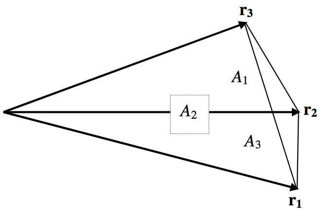
\(\text{FIGURE XIII.1}\)
Figure \(\text{XIII.1}\) shows three coplanar vectors. It is clearly possible to express \(\textbf{r}_2\) as a linear combination of the other two. That is to say, it should be possible to find coefficients such that
\[\textbf{r}_2 = a_1 \textbf{r}_1 + a_3 \textbf{r}_3 . \label{13.2.1}\]
The notation I am going to use is as follows:
- The area of the triangle formed by joining the tips of \(\textbf{r}_2\) and \(\textbf{r}_3\) is \(A_1\).
- The area of the triangle formed by joining the tips of \(\textbf{r}_3\) and \(\textbf{r}_1\) is \(A_2\).
- The area of the triangle formed by joining the tips of \(\textbf{r}_1\) and \(\textbf{r}_2\) is \(A_3\).
To find the coefficients in Equation \ref{13.2.1}, multiply both sides by \(\textbf{r}_1 \times\):
\[\textbf{r}_1 \times \textbf{r}_2 = a_3 \textbf{r}_1 \times \textbf{r}_3 . \label{13.2.2}\]
The two vector products are parallel vectors (they are each perpendicular to the plane of the paper), of magnitudes \(2A_3\) and \(2A_2\) respectively. (\(2A_3\) is the area of the parallelogram of which the vectors \(\textbf{r}_1\) and \(\textbf{r}_2\) form two sides.)
\[\therefore a_3 = A_3/A_2 . \label{13.2.3}\]
Similarly by multiplying both sides of Equation \ref{13.2.1} by \(\textbf{r}_3 \times\) it will be found that
\[a_1 = A_1/ A_2 . \label{13.2.4}\]
Hence we find that
\[A_2 \textbf{r}_2 = A_1 \textbf{r}_1 + A_3 \textbf{r}_3 . \label{13.2.5}\]