
11.2: Standard Coordinates and Plate Constants


- Last updated
- Mar 5, 2022
- Save as PDF

( \newcommand{\kernel}{\mathrm{null}\,}\)
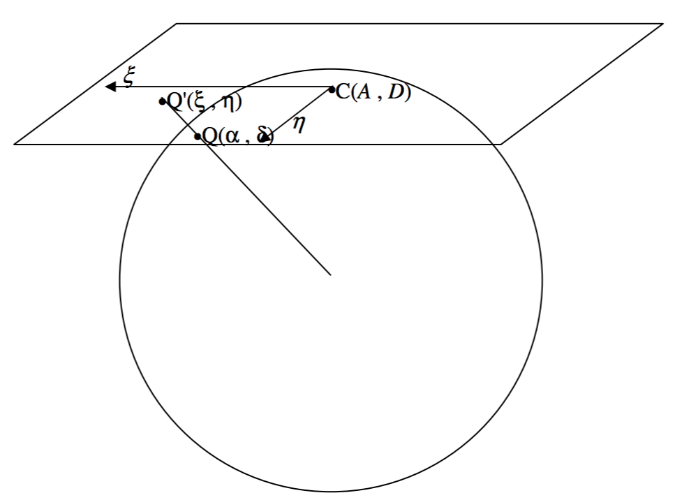
We shall suppose that the optic axis of the telescope, whose effective focal length is F, is pointing to a point \text{C} on the celestial sphere, whose right ascension and declination are (A, \ D). The stars, as every astrophysicist knows, are scattered around on the surface of the celestial sphere, which is of arbitrary radius, and I shall take the radius to be equal to F, the focal length of the telescope. In figure \text{XI.1}, I have drawn the tangent plane to the sky at \text{C}, which is what will be recorded on the photograph. In the tangent plane (which is similar to the plane of the photographic plate or film) I have drawn two orthogonal axes: \text{C}ξ to the east and \text{C}η to the north. I have drawn a star, \text{Q}, whose coordinates are (α,δ), on the surface of the celestial sphere, and its projection, \text{Q}^\prime, on the tangent plane, where its coordinates are (ξ , η). Every star is similarly mapped on to the tangent plane by a similar projection. The coordinates (ξ , η) are called the standard coordinates of the star, and our first task is to find a relation between the equatorial coordinates (α,δ) on the surface of the celestial sphere and the standard coordinates (ξ , η) on the tangent plane or the photograph.
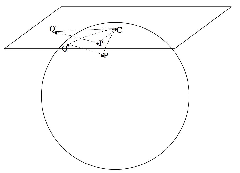
In figure \text{XI.2}, I have re-drawn figure \text{XI.1}, and, in addition to the star \text{Q} and its projection \text{Q}^\prime, I have also drawn the north Celestial Pole \text{P} and its projection \text{P}^\prime. The point \text{P}^\prime is on the η axis. The spherical triangle \text{PQC} maps onto the plane triangle \text{P}^\prime \text{Q}^\prime \text{C}. On the spherical triangle \text{PQC}, the side \text{PQ} = 90^\circ − δ and the side \text{PC} = 90^\circ − D.
\text{FIGURE XI.1}
\text{FIGURE XI.1}
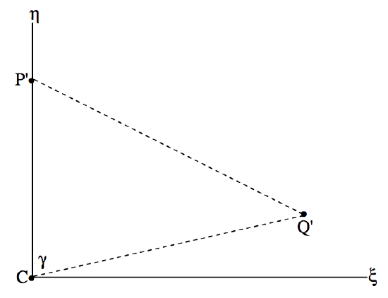
The angle \text{PCQ} in the spherical triangle \text{PCQ} is equal to the angle \text{P}^\prime \text{CQ}^\prime in the plane triangle \text{P}^\prime \text{CQ}^\prime, and I shall call that angle γ. I shall call the arc \text{CQ} in the spherical triangle ε. In figure \text{XI.3} I draw the tangent plane, showing the ξ- and η-axes and the projections, \text{P}^\prime and \text{Q}^\prime of the pole \text{P} and the star \text{Q}, as well as the plane triangle \text{P}^\prime \text{CQ}^\prime.
\text{FIGURE XI.3}
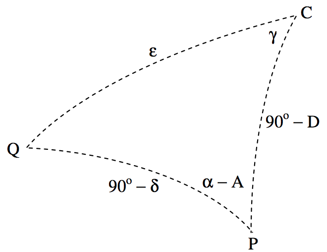
The ξ and η coordinates of \text{Q}^\prime are (\text{CQ}^\prime \sin γ , \ \text{CQ}^\prime \cos γ). And by staring at figures \text{XI.1} and \text{XI.2} for a while, you can see that \text{CQ}^\prime = F \tan ε. Thus the standard coordinate of the image \text{Q}^\prime of the star on the photograph, in units of the focal length of the telescope, are (\tan ε \sin γ , \ \tan ε \cos γ ). It remains now to find expressions for \tan ε \sin γ and \tan ε \cos γ in terms of the right ascensions and declinations of \text{Q} and of \text{C}. I draw now, in figure \text{XI.4}, the spherical triangle \text{PCQ}.
\text{FIGURE XI.4}
It is easy, from the usual formulas for spherical triangles, to obtain expressions for \cos ε and for \tan γ :
\cos ε = \sin δ \sin D + \cos δ \cos D \cos (α - A) \label{11.2.1} \tag{11.2.1}
and
\tan γ = \frac{\sin (α - A)}{\cos D \tan δ - \sin D \cos (α - A)}, \label{11.2.2} \tag{11.2.2}
from which one can (eventually) calculate the standard coordinates (ξ , η) of the star. It is also possible to calculate explicit expressions for \tan ε \sin γ and for \tan ε \cos γ. Thus, by further applications of the spherical triangle formulas, we have
\tan ε = \frac{\cos D}{\sin D \cos γ + \cot (α - A) \sin γ}. \label{11.2.3} \tag{11.2.3}
Multiplication of Equation \ref{11.2.3} by \sin γ gives \tan ε \sin γ except that \tan γ appears on the right hand side. This, however, can be eliminated by use of Equation \ref{11.2.2}, and one obtains, after some algebra:
ξ = \tan ε \sin γ = \frac{\sin (α - A)}{\sin D \tan δ + \cos D \cos (α - A)}. \label{11.2.4} \tag{11.2.4}
In a similar way, you can multiply Equation \text{11.2.3} by \cos γ, and again eliminate \tan γ and eventually arrive at
η = \tan ε \cos γ = \frac{\tan δ - \tan D \cos (α - A)}{\tan D \tan δ + \cos(α - A)}. \label{11.2.5} \tag{11.2.5}
These give the standard coordinates of a star or asteroid at (α , δ) in units of the focal length F.
Now it would seem that all we have to do is to measure the standard coordinates (ξ , η) of an object, and we can immediately determine its right ascension and declination by inverting Equations \ref{11.2.4} and \ref{11.2.5}:
\tan(α - A) = \frac{ξ}{\cos D - η \sin D} \label{11.2.6} \tag{11.2.6}
and
\tan δ = \frac{(η \cos D + \sin D)\sin(α - A)}{ξ}. \label{11.2.7} \tag{11.2.7}
Indeed in principle that is what we have to do – but in practice we are still some way from achieving our aim.
One small difficulty is that we do not know the effective focal length F (which depends on the temperature) precisely. A more serious problem is that we do not know the exact position of the plate centre, nor do we know that the directions of travel of our two-coordinate measuring engine are parallel to the directions of right ascension and declination.
The best we can do is to start our measurements from some point near the plate centre and measure (in mm rather than in units of F) the horizontal and vertical distances (x , y) of the comparison stars and the asteroid from our arbitrary origin. These (x , y) coordinates are called, naturally, the measured coordinates.
The measured coordinates will usually be expressed in millimetres (or perhaps in pixels if a CCD is being used), and the linear distance s between any two comparison star images is found by the theorem of Pythagoras. The angular distance ω between any two stars is given by solution of a spherical triangle as
\cos ω = \sin δ_1 \sin δ_2 + \cos δ_1 \cos δ_2 \cos (α_1 - α_2) \label{11.2.8} \tag{11.2.8}
The focal length F is then s/ω, and this can be calculated for several pairs of stars and averaged. From that point the standard coordinates can then be expressed in units of F.
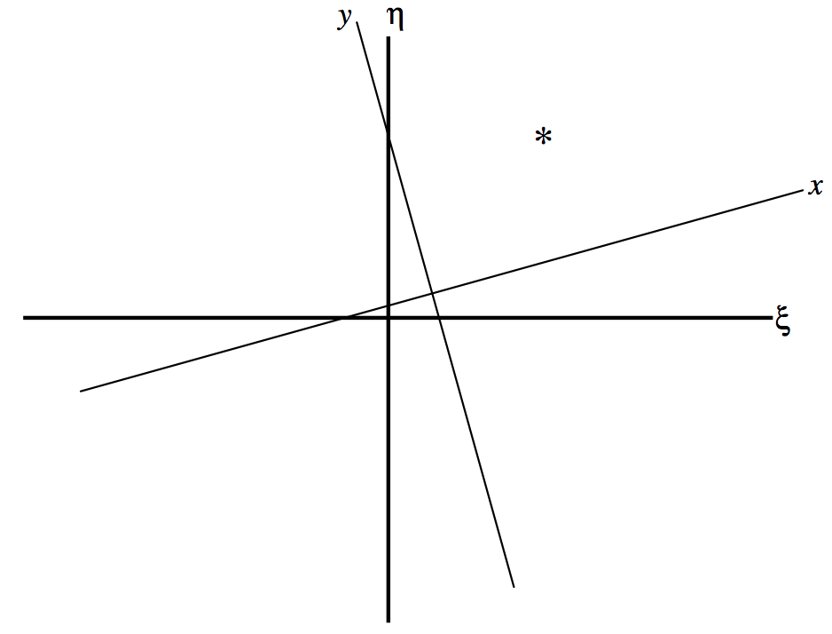
The measured coordinates (x , y) are displaced from the standard coordinates (ξ , η) by an unknown translation and an unknown rotation (figure \text{XI.4}) , but the relation between them, if unknown, is at least linear (but see subsection \text{11.3.5}) and thus of the form:
ξ - x = ax + by + c, \label{11.2.9} \tag{11.2.9}
η - y = dx + ey + f . \label{11.2.10} \tag{11.2.10}
The constants a – f are the plate constants. They are determined by measuring the standard coordinates for a minimum of three comparison stars whose right ascensions and declinations are known and for which the standard coordinates can therefore be calculated. Three sets of Equations \ref{11.2.9} and 10 can then be set up and solved for the plate constants. In practice more than three comparison stars should be chosen, and a least squares solution determined. For how to do this, see either section 8 of chapter 1, or the article cited in section 1 of this chapter. In the photographic days, just a few (perhaps half a dozen) comparison stars were used. Today, when there are catalogues containing hundreds of millions of stars, and \text{CCD} measurement and automatic computation are so much faster, several dozen comparison stars may be used, and any poor measurements (or poor catalogue positions) can quickly be identified and rejected.
Having determined the plate constants, Equations \ref{11.2.9} and 10 can be used to calculate the standard coordinates of the asteroid, and hence its right ascension and declination can be calculated from Equations \ref{11.2.6} and 7.
\text{FIGURE 11.5}
It should be noted that the position of the asteroid that you have measured – and should report to the Minor Planet Center, is the topocentric position (i.e. as measured from your position on the surface of Earth) rather than the geocentric position (as seen from the centre of Earth). The Minor Planet Center expects to receive from the observer the topocentric position; the MPC will know how to make the correction to the centre of Earth.