
11.4: Curve of Growth for Gaussian Profiles


- Last updated
- Mar 5, 2022
- Save as PDF

( \newcommand{\kernel}{\mathrm{null}\,}\)
By “gaussian profile” in the title of this section, I mean profiles that are gaussian in the optically-thin case; as soon as there are departures from optical thinness, there are also departures from the gaussian profile. Alternatively, the absorption coefficient and the optical depth are gaussian; the absorptance is not.
For an optically-thin thermally-broadened line, the optical thickness as a function of wavelength is given by
τ(x)=τ(0)exp(−x2ln2g2),
where the HWHM is
g=Vmλ0√ln2c.
Here Vm is the modal speed. (See Chapter 10 for details.) The line profiles, as calculated from equations 11.3.4 and ???, are shown in figure XI.2 for the following values of the optical thickness at the line centre: τ(0)=116,18,14,12,1,2,4,8.
On combining equations 11.3.4 and ??? and ???, we obtain the following expression for the equivalent width:
W=2∫∞0(1−exp{−τ(0)e−x2ln2/g2})dx,
or
W=2Vmλ0c∫∞0(1−exp{−τ(0)e−Δ2})dΔ,
where
Δ=x√ln2g=cxVmλ0.
The half-width at half maximum (HWHM) of the expression ??? for the optical thickness corresponds to Δ=√ln2=0.8326. For the purposes of practical numerical integration of Equation ???, I shall integrate from Δ=−5 to +5 that is to say from ±6 times the HWHm. One can appreciate from figure XI.2 that going outside these limits will not contribute significantly to the equivalent width. I shall calculate the equivalent width for central optical depths ranging from 1/20(logτ(0)=−1.3) to 105(logτ(0)=5.0).
What we have in figure XI.3 is a curve of growth for thermally broadened lines (or lines that, in the optically thin limit, have a gaussian profile, which could include a thermal and a microturbulent component). I have plotted this from logτ(0)=−1.3 to +5.0; that is τ(0)=0.05 to 105.
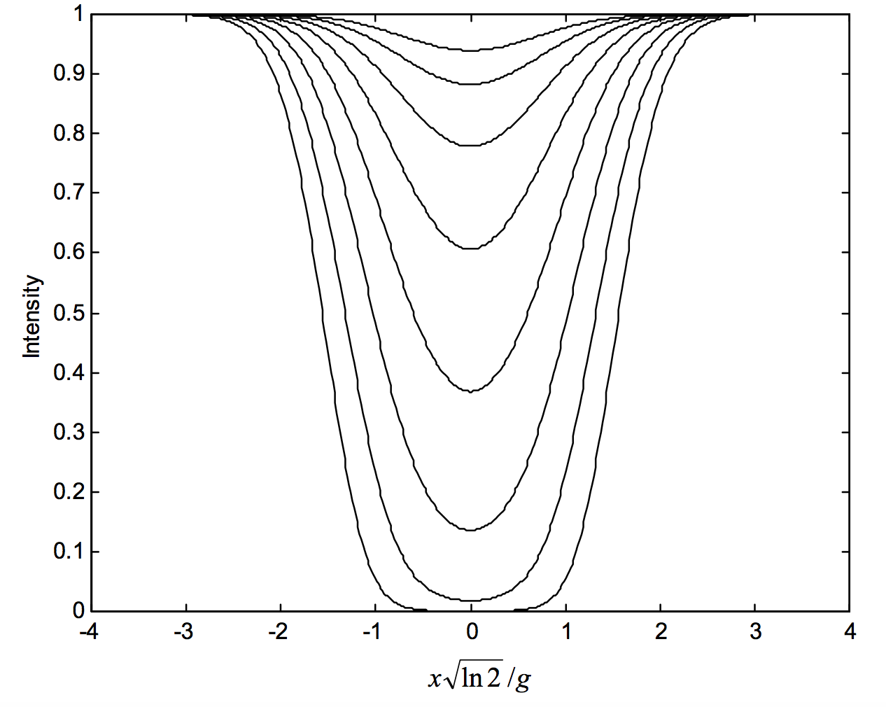
FIGURE XI.2
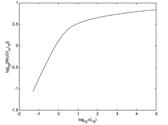
FIGURE XI.3