
18.4: Worked Examples
- Page ID
- 24539
\( \newcommand{\vecs}[1]{\overset { \scriptstyle \rightharpoonup} {\mathbf{#1}} } \)
\( \newcommand{\vecd}[1]{\overset{-\!-\!\rightharpoonup}{\vphantom{a}\smash {#1}}} \)
\( \newcommand{\dsum}{\displaystyle\sum\limits} \)
\( \newcommand{\dint}{\displaystyle\int\limits} \)
\( \newcommand{\dlim}{\displaystyle\lim\limits} \)
\( \newcommand{\id}{\mathrm{id}}\) \( \newcommand{\Span}{\mathrm{span}}\)
( \newcommand{\kernel}{\mathrm{null}\,}\) \( \newcommand{\range}{\mathrm{range}\,}\)
\( \newcommand{\RealPart}{\mathrm{Re}}\) \( \newcommand{\ImaginaryPart}{\mathrm{Im}}\)
\( \newcommand{\Argument}{\mathrm{Arg}}\) \( \newcommand{\norm}[1]{\| #1 \|}\)
\( \newcommand{\inner}[2]{\langle #1, #2 \rangle}\)
\( \newcommand{\Span}{\mathrm{span}}\)
\( \newcommand{\id}{\mathrm{id}}\)
\( \newcommand{\Span}{\mathrm{span}}\)
\( \newcommand{\kernel}{\mathrm{null}\,}\)
\( \newcommand{\range}{\mathrm{range}\,}\)
\( \newcommand{\RealPart}{\mathrm{Re}}\)
\( \newcommand{\ImaginaryPart}{\mathrm{Im}}\)
\( \newcommand{\Argument}{\mathrm{Arg}}\)
\( \newcommand{\norm}[1]{\| #1 \|}\)
\( \newcommand{\inner}[2]{\langle #1, #2 \rangle}\)
\( \newcommand{\Span}{\mathrm{span}}\) \( \newcommand{\AA}{\unicode[.8,0]{x212B}}\)
\( \newcommand{\vectorA}[1]{\vec{#1}} % arrow\)
\( \newcommand{\vectorAt}[1]{\vec{\text{#1}}} % arrow\)
\( \newcommand{\vectorB}[1]{\overset { \scriptstyle \rightharpoonup} {\mathbf{#1}} } \)
\( \newcommand{\vectorC}[1]{\textbf{#1}} \)
\( \newcommand{\vectorD}[1]{\overrightarrow{#1}} \)
\( \newcommand{\vectorDt}[1]{\overrightarrow{\text{#1}}} \)
\( \newcommand{\vectE}[1]{\overset{-\!-\!\rightharpoonup}{\vphantom{a}\smash{\mathbf {#1}}}} \)
\( \newcommand{\vecs}[1]{\overset { \scriptstyle \rightharpoonup} {\mathbf{#1}} } \)
\(\newcommand{\longvect}{\overrightarrow}\)
\( \newcommand{\vecd}[1]{\overset{-\!-\!\rightharpoonup}{\vphantom{a}\smash {#1}}} \)
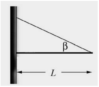
\(\newcommand{\avec}{\mathbf a}\) \(\newcommand{\bvec}{\mathbf b}\) \(\newcommand{\cvec}{\mathbf c}\) \(\newcommand{\dvec}{\mathbf d}\) \(\newcommand{\dtil}{\widetilde{\mathbf d}}\) \(\newcommand{\evec}{\mathbf e}\) \(\newcommand{\fvec}{\mathbf f}\) \(\newcommand{\nvec}{\mathbf n}\) \(\newcommand{\pvec}{\mathbf p}\) \(\newcommand{\qvec}{\mathbf q}\) \(\newcommand{\svec}{\mathbf s}\) \(\newcommand{\tvec}{\mathbf t}\) \(\newcommand{\uvec}{\mathbf u}\) \(\newcommand{\vvec}{\mathbf v}\) \(\newcommand{\wvec}{\mathbf w}\) \(\newcommand{\xvec}{\mathbf x}\) \(\newcommand{\yvec}{\mathbf y}\) \(\newcommand{\zvec}{\mathbf z}\) \(\newcommand{\rvec}{\mathbf r}\) \(\newcommand{\mvec}{\mathbf m}\) \(\newcommand{\zerovec}{\mathbf 0}\) \(\newcommand{\onevec}{\mathbf 1}\) \(\newcommand{\real}{\mathbb R}\) \(\newcommand{\twovec}[2]{\left[\begin{array}{r}#1 \\ #2 \end{array}\right]}\) \(\newcommand{\ctwovec}[2]{\left[\begin{array}{c}#1 \\ #2 \end{array}\right]}\) \(\newcommand{\threevec}[3]{\left[\begin{array}{r}#1 \\ #2 \\ #3 \end{array}\right]}\) \(\newcommand{\cthreevec}[3]{\left[\begin{array}{c}#1 \\ #2 \\ #3 \end{array}\right]}\) \(\newcommand{\fourvec}[4]{\left[\begin{array}{r}#1 \\ #2 \\ #3 \\ #4 \end{array}\right]}\) \(\newcommand{\cfourvec}[4]{\left[\begin{array}{c}#1 \\ #2 \\ #3 \\ #4 \end{array}\right]}\) \(\newcommand{\fivevec}[5]{\left[\begin{array}{r}#1 \\ #2 \\ #3 \\ #4 \\ #5 \\ \end{array}\right]}\) \(\newcommand{\cfivevec}[5]{\left[\begin{array}{c}#1 \\ #2 \\ #3 \\ #4 \\ #5 \\ \end{array}\right]}\) \(\newcommand{\mattwo}[4]{\left[\begin{array}{rr}#1 \amp #2 \\ #3 \amp #4 \\ \end{array}\right]}\) \(\newcommand{\laspan}[1]{\text{Span}\{#1\}}\) \(\newcommand{\bcal}{\cal B}\) \(\newcommand{\ccal}{\cal C}\) \(\newcommand{\scal}{\cal S}\) \(\newcommand{\wcal}{\cal W}\) \(\newcommand{\ecal}{\cal E}\) \(\newcommand{\coords}[2]{\left\{#1\right\}_{#2}}\) \(\newcommand{\gray}[1]{\color{gray}{#1}}\) \(\newcommand{\lgray}[1]{\color{lightgray}{#1}}\) \(\newcommand{\rank}{\operatorname{rank}}\) \(\newcommand{\row}{\text{Row}}\) \(\newcommand{\col}{\text{Col}}\) \(\renewcommand{\row}{\text{Row}}\) \(\newcommand{\nul}{\text{Nul}}\) \(\newcommand{\var}{\text{Var}}\) \(\newcommand{\corr}{\text{corr}}\) \(\newcommand{\len}[1]{\left|#1\right|}\) \(\newcommand{\bbar}{\overline{\bvec}}\) \(\newcommand{\bhat}{\widehat{\bvec}}\) \(\newcommand{\bperp}{\bvec^\perp}\) \(\newcommand{\xhat}{\widehat{\xvec}}\) \(\newcommand{\vhat}{\widehat{\vvec}}\) \(\newcommand{\uhat}{\widehat{\uvec}}\) \(\newcommand{\what}{\widehat{\wvec}}\) \(\newcommand{\Sighat}{\widehat{\Sigma}}\) \(\newcommand{\lt}{<}\) \(\newcommand{\gt}{>}\) \(\newcommand{\amp}{&}\) \(\definecolor{fillinmathshade}{gray}{0.9}\)Example 18.2 Suspended Rod
A uniform rod of length \(l=2.0 \mathrm{m}\) and mass \(m=4.0 \mathrm{kg}\) is hinged to a wall at one end and suspended from the wall by a cable that is attached to the other end of the rod at an angle of \(\beta=30^{\circ}\) to the rod (see Figure 18.7). Assume the cable has zero mass. There is a contact force at the pivot on the rod. The magnitude and direction of this force is unknown. One of the most difficult parts of these types of problems is to introduce an angle for the pivot force and then solve for that angle if possible. In this problem you will solve for the magnitude of the tension in the cable and the direction and magnitude of the pivot force. (a) What is the tension in the cable? (b) What angle does the pivot force make with the beam? (c) What is the magnitude of the pivot force?
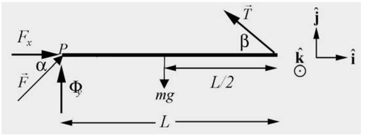
Solution: a) The force diagram is shown in Figure 18.8. Take the positive \(\hat{\mathbf{i}}\)-direction to be to the right in the figure above, and take the positive \(\hat{\mathbf{j}}\)-direction to be vertically upward. The forces on the rod are: the gravitational force \(m \overrightarrow{\mathbf{g}}=-m g \hat{\mathbf{j}}\), acting at the center of the rod; the force that the cable exerts on the rod, \(\overrightarrow{\mathbf{T}}=T(-\cos \beta \hat{\mathbf{i}}+\sin \beta \hat{\mathbf{j}})\) acting at the right end of the rod; and the pivot force \(\overrightarrow{\mathbf{F}}_{\text {pivot }}=F(\cos \alpha \hat{\mathbf{i}}+\sin \alpha \hat{\mathbf{j}})\), acting at pivot the left end of the rod. If \(0<\alpha<\pi / 2\) the pivot force is directed up and to the right in the figure. If \(0>\alpha>-\pi / 2\), the pivot force is directed down and to the right. We have no reason, at this point, to expect that \(\alpha\) will be in either of the quadrants, but it must be in one or the other.
will be in either of the quadrants, but it must be in one or the other
\[\begin{array}{l}
0=-T \cos \beta+F \cos \alpha \\
0=-m g+T \sin \beta+F \sin \alpha
\end{array} \nonumber \]
With respect to the pivot point, and taking positive torques to be counterclockwise, the gravitational force exerts a negative torque of magnitude \(m g(l / 2)\) and the cable exerts a positive torque of magnitude \(T l \sin \beta\). The pivot force exerts no torque about the pivot. Setting the sum of the torques equal to zero then gives
\[\begin{array}{l}
0=T l \sin \beta-m g(l / 2) \\
T=\frac{m g}{2 \sin \beta}
\end{array} \nonumber \]
This result has many features we would expect; proportional to the weight of the rod and inversely proportional to the sine of the angle made by the cable with respect to the horizontal. Inserting numerical values gives
\[T=\frac{m g}{2 \sin \beta}=\frac{(4.0 \mathrm{kg})\left(9.8 \mathrm{m} \cdot \mathrm{s}^{-2}\right)}{2 \sin 30^{\circ}}=39.2 \mathrm{N} \nonumber \]
There are many ways to find the angle \(\alpha\). Substituting Equation (18.4.2) for the tension into both force equations in Equation (18.4.1) yields
\[\begin{array}{l}
F \cos \alpha=T \cos \beta=(m g / 2) \cot \beta \\
F \sin \alpha=m g-T \sin \beta=m g / 2
\end{array} \nonumber \]
In Equation (18.4.4), dividing one equation by the other, we see that \(\tan \alpha=\tan \beta, \alpha=\beta\)
The horizontal forces on the rod must cancel. The tension force and the pivot force act with the same angle (but in opposite horizontal directions) and hence must have the same magnitude,
\[F=T=39.2 \mathrm{N} \nonumber \]
As an alternative, if we had not done the previous parts, we could find torques about the point where the cable is attached to the wall. The cable exerts no torque about this point and the y -component of the pivot force exerts no torque as well. The moment arm of the x -component of the pivot force is \(l \tan \beta\) and the moment arm of the weight is l / 2 . Equating the magnitudes of these two torques gives
\[F \cos \alpha l \tan \beta=m g \frac{l}{2} \nonumber \]
equivalent to the first equation in Equation (18.4.4). Similarly, evaluating torques about the right end of the rod, the cable exerts no torques and the x -component of the pivot force exerts no torque. The moment arm of the y -component of the pivot force is l and the moment arm of the weight is l / 2 . Equating the magnitudes of these two torques gives
\[F \sin \alpha l=m g \frac{l}{2} \nonumber \]
reproducing the second equation in Equation (18.4.4). The point of this alternative solution is to show that choosing a different origin (or even more than one origin) in order to remove an unknown force from the torques equations might give a desired result more directly.
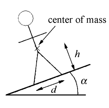
Example 18.3 Person Standing on a Hill
A person is standing on a hill that is sloped at an angle of \(\alpha\) with respect to the horizontal (Figure 18.9). The person’s legs are separated by a distance \(d\), with one foot uphill and one downhill. The center of mass of the person is at a distance \(h\) above the ground, perpendicular to the hillside, midway between the person’s feet. Assume that the coefficient of static friction between the person’s feet and the hill is sufficiently large that the person will not slip. (a) What is the magnitude of the normal force on each foot? (b) How far must the feet be apart so that the normal force on the upper foot is just zero? This is the moment when the person starts to rotate and fall over.
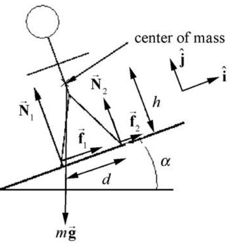
Solution: The force diagram on the person is shown in Figure 18.10. Note that the contact forces have been decomposed into components perpendicular and parallel to the hillside. A choice of unit vectors and positive direction for torque is also shown. Applying Newton’s Second Law to the two components of the net force,
\[\hat{\mathbf{j}}: N_{1}+N_{2}-m g \cos \alpha=0 \nonumber \]
\[\hat{\mathbf{i}}: f_{1}+f_{2}-m g \sin \alpha=0 \nonumber \]
These two equations imply that
\[N_{1}+N_{2}=m g \cos \alpha \nonumber \]
\[f_{1}+f_{2}=m g \sin \alpha \nonumber \]
Evaluating torques about the center of mass,
\[h\left(f_{1}+f_{2}\right)+\left(N_{2}-N_{1}\right) \frac{d}{2}=0 \nonumber \]
Equation (18.4.10) can be rewritten as
\[N_{1}-N_{2}=\frac{2 h\left(f_{1}+f_{2}\right)}{d} \nonumber \]
Substitution of Equation (18.4.9) into Equation (18.4.11) yields
\[N_{1}-N_{2}=\frac{2 h(m g \sin \alpha)}{d} \nonumber \]
We can solve for \(N_{1}\) by adding Equations (18.4.8) and (18.4.12), and then dividing by 2, yielding
\[N_{1}=\frac{1}{2} m g \cos \alpha+\frac{h(m g \sin \alpha)}{d}=m g\left(\frac{1}{2} \cos \alpha+\frac{h}{d} \sin \alpha\right) \nonumber \]
Similarly, we can solve for \(N_{2}\) by subtracting Equation (18.4.12) from Equation (18.4.8) and dividing by 2, yielding
\[N_{2}=m g\left(\frac{1}{2} \cos \alpha-\frac{h}{d} \sin \alpha\right) \nonumber \]
The normal force \(N_{2}\) as given in Equation (18.4.14) vanishes when
\[\frac{1}{2} \cos \alpha=\frac{h}{d} \sin \alpha \nonumber \]
which can be solved for the minimum distance between the legs,
\[d=2 h(\tan \alpha) \nonumber \]
It should be noted that no specific model for the frictional force was used, that is, no coefficient of static friction entered the problem. The two frictional forces \(f_{1}\) and \(f_{2}\) were not determined separately; only their sum entered the above calculations.
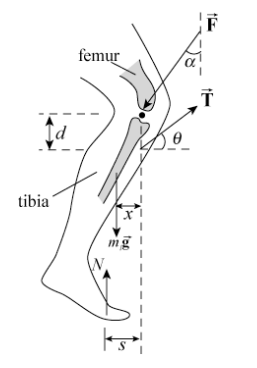
Example 18.4 The Knee
A man of mass m = 70 kg is about to start a race. Assume the runner’s weight is equally distributed on both legs. The patellar ligament in the knee is attached to the upper tibia and runs over the kneecap. When the knee is bent, a tensile force, \(\overrightarrow{\mathbf{T}}\), that the ligament exerts on the upper tibia, is directed at an angle of \(\theta=40^{\circ}\) with respect to the horizontal. The femur exerts a force \(\overrightarrow{\mathbf{F}}\) on the upper tibia. The angle, \(\alpha\) that this force makes with the vertical will vary and is one of the unknowns to solve for. Assume that the ligament is connected a distance, \(d=3.8 \mathrm{cm}\), directly below the contact point of the femur on the tibia. The contact point between the foot and the ground is a distance \(s=3.6 \times 10^{1} \mathrm{cm}\) from the vertical line passing through contact point of the femur on the tibia. The center of mass of the lower leg lies a distance \(x=1.8 \times 10^{1} \mathrm{cm}\) from this same vertical line. Suppose the mass \(m_{\mathrm{L}}\) of the lower leg is a 1/10 of the mass of the body (Figure 18.11). (a) Find the magnitude T of the force \(\overrightarrow{\mathbf{T}}\) of the patellar ligament on the tibia. (b) Find the direction (the angle α ) of the force \(\overrightarrow{\mathbf{F}}\) of the femur on the tibia. (c) Find the magnitude F of the force \(\overrightarrow{\mathbf{F}}\) of the femur on the tibia.
Solutions: a) Choose the unit vector \(\hat{\mathbf{i}}\) to be directed horizontally to the right and \(\hat{\mathbf{j}}\) directed vertically upwards. The first condition for static equilibrium, Equation (18.1.1), that the sum of the forces is zero becomes
\[\hat{\mathbf{i}}:-F \sin \alpha+T \cos \theta=0 \nonumber \]
\[\hat{\mathbf{j}}: N-F \cos \alpha+T \sin \theta-(1 / 10) m g=0 \nonumber \]
Because the weight is evenly distributed on the two feet, the normal force on one foot is equal to half the weight, or
\[N=(1 / 2) m g \nonumber \]
Equation (18.4.18) becomes
\[\begin{array}{r}
\hat{\mathbf{j}}:(1 / 2) m g-F \cos \alpha+T \sin \theta-(1 / 10) m g=0 \\
(2 / 5) m g-F \cos \alpha+T \sin \theta=0
\end{array} \nonumber \]
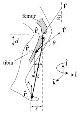
The torque-force diagram on the knee is shown in Figure 18.12. Choose the point of action of the ligament on the tibia as the point \(S\) about which to compute torques. Note that the tensile force, \(\overrightarrow{\mathbf{T}}\) that the ligament exerts on the upper tibia will make no contribution to the torque about this point \(S\). This may help slightly in doing the calculations. Choose counterclockwise as the positive direction for the torque; this is the positive \(\hat{\mathbf{k}}\)- direction. Then the torque due to the force \(\overrightarrow{\mathbf{F}}\) of the femur on the tibia is
\[\vec{\tau}_{S, 1}=\overrightarrow{\mathbf{r}}_{S, 1} \times \overrightarrow{\mathbf{F}}=d \hat{\mathbf{j}} \times(-F \sin \alpha \hat{\mathbf{i}}-F \cos \alpha \hat{\mathbf{j}})=d F \sin \alpha \hat{\mathbf{k}} \nonumber \]
The torque due to the mass of the leg is
\[\vec{\tau}_{S, 2}=\overrightarrow{\mathbf{r}}_{S, 2} \times(-m g / 10) \hat{\mathbf{j}}=\left(-x \hat{\mathbf{i}}-y_{L} \hat{\mathbf{j}}\right) \times(-m g / 10) \hat{\mathbf{j}}=(1 / 10) x m g \hat{\mathbf{k}} \nonumber \]
The torque due to the normal force of the ground is
\[\vec{\tau}_{S, 3}=\overrightarrow{\mathbf{r}}_{S, 3} \times N \hat{\mathbf{j}}=\left(-s \hat{\mathbf{i}}-y_{N} \hat{\mathbf{j}}\right) \times N \hat{\mathbf{j}}=-s N \hat{\mathbf{k}}=-(1 / 2) s m g \hat{\mathbf{k}} \nonumber \]
(In Equations (18.4.22) and (18.4.23), \(y_{L} \text { and } y_{N}\) are the vertical displacements of the τ point where the weight of the leg and the normal force with respect to the point S; as can be seen, these quantities do not enter directly into the calculations.) The condition that the sum of the torques about the point \(S\) vanishes, Equation (18.1.2),
\[\vec{\tau}_{S, \text { total }}=\vec{\tau}_{S, 1}+\vec{\tau}_{S, 2}+\vec{\tau}_{S, 3}=\overrightarrow{0} \nonumber \]
becomes
\[d F \sin \alpha \hat{\mathbf{k}}+(1 / 10) x m g \hat{\mathbf{k}}-(1 / 2) s m g \hat{\mathbf{k}}=\overrightarrow{\boldsymbol{0}} \nonumber \]
The three equations in the three unknowns are summarized below:
\[\begin{array}{r}
-F \sin \alpha+T \cos \theta=0 \\
(2 / 5) m g-F \cos \alpha+T \sin \theta=0 \\
d F \sin \alpha+(1 / 10) x m g-(1 / 2) s m g=0
\end{array} \nonumber \]
The horizontal force equation, the first in (18.4.26), implies that
\[F \sin \alpha=T \cos \theta \nonumber \]
Substituting this into the torque equation, the third equation of (18.4.26), yields
\[d T \cos \theta+(1 / 10) x m g-s(1 / 2) m g=0 \nonumber \]
Note that Equation (18.4.28) is the equation that would have been obtained if we had chosen the contact point between the tibia and the femur as the point about which to determine torques. Had we chosen this point, we would have saved one minor algebraic step. We can solve this Equation (18.4.28) for the magnitude T of the force \(\overrightarrow{\mathbf{T}}\) of the patellar ligament on the tibia,
\[T=\frac{s(1 / 2) m g-(1 / 10) x m g}{d \cos \theta} \nonumber \]
Inserting numerical values into Equation (18.4.29),
\[\begin{aligned}
T &=(70 \mathrm{kg})\left(9.8 \mathrm{m} \cdot \mathrm{s}^{-2}\right) \frac{\left(3.6 \times 10^{-1} \mathrm{m}\right)(1 / 2)-(1 / 10)\left(1.8 \times 10^{-1} \mathrm{m}\right)}{\left(3.8 \times 10^{-2} \mathrm{m}\right) \cos \left(40^{\circ}\right)} \\
&=3.8 \times 10^{3} \mathrm{N}
\end{aligned} \nonumber \]
b) We can now solve for the direction \(\alpha\) of the force \(\overrightarrow{\mathbf{F}}\) of the femur on the tibia as follows. Rewrite the two force equations in (18.4.26) as
\[\begin{array}{l}
F \cos \alpha=(2 / 5) m g+T \sin \theta \\
F \sin \alpha=T \cos \theta
\end{array} \nonumber \]
Dividing these equations yields
\[\frac{F \cos \alpha}{F \sin \alpha}=\operatorname{cotan} \alpha=\frac{(2 / 5) m g+T \sin \theta}{T \cos \theta} \nonumber \]
And so
\[\begin{array}{l}
\alpha=\operatorname{cotan}^{-1}\left(\frac{(2 / 5) m g+T \sin \theta}{T \cos \theta}\right) \\
\alpha=\operatorname{cotan}^{-1}\left(\frac{(2 / 5)(70 \mathrm{kg})\left(9.8 \mathrm{m} \cdot \mathrm{s}^{-2}\right)+\left(3.4 \times 10^{3} \mathrm{N}\right) \sin \left(40^{\circ}\right)}{\left(3.4 \times 10^{3} \mathrm{N}\right) \cos \left(40^{\circ}\right)}\right)=47^{\circ}
\end{array} \nonumber \]
c) We can now use the horizontal force equation to calculate the magnitude F of the force of the femur \(\overrightarrow{\mathbf{F}}\) on the tibia from Equation (18.4.27),
\[F=\frac{\left(3.8 \times 10^{3} \mathrm{N}\right) \cos \left(40^{\circ}\right)}{\sin \left(47^{\circ}\right)}=4.0 \times 10^{3} \mathrm{N} \nonumber \]
Note you can find a symbolic expression for \(\alpha\) that did not involve the intermediate numerical calculation of the tension. This is rather complicated algebraically; basically, the last two equations in (18.4.26) are solved for F and T in terms of \(\alpha, \theta\) and the other variables (Cramer’s Rule is suggested) and the results substituted into the first of (18.4.26). The resulting expression is
\[\begin{aligned}
\cot \alpha &=\frac{(s / 2-x / 10) \sin \left(40^{\circ}\right)+\left((2 d / 5) \cos \left(40^{\circ}\right)\right)}{(s / 2-x / 10) \cos \left(40^{\circ}\right)} \\
&=\tan \left(40^{\circ}\right)+\frac{2 d / 5}{s / 2-x / 10}
\end{aligned} \nonumber \]
which leads to the same numerical result, \(\alpha=47^{\circ}\)