
28.3: Mass Continuity Equation
- Page ID
- 25565
\( \newcommand{\vecs}[1]{\overset { \scriptstyle \rightharpoonup} {\mathbf{#1}} } \)
\( \newcommand{\vecd}[1]{\overset{-\!-\!\rightharpoonup}{\vphantom{a}\smash {#1}}} \)
\( \newcommand{\dsum}{\displaystyle\sum\limits} \)
\( \newcommand{\dint}{\displaystyle\int\limits} \)
\( \newcommand{\dlim}{\displaystyle\lim\limits} \)
\( \newcommand{\id}{\mathrm{id}}\) \( \newcommand{\Span}{\mathrm{span}}\)
( \newcommand{\kernel}{\mathrm{null}\,}\) \( \newcommand{\range}{\mathrm{range}\,}\)
\( \newcommand{\RealPart}{\mathrm{Re}}\) \( \newcommand{\ImaginaryPart}{\mathrm{Im}}\)
\( \newcommand{\Argument}{\mathrm{Arg}}\) \( \newcommand{\norm}[1]{\| #1 \|}\)
\( \newcommand{\inner}[2]{\langle #1, #2 \rangle}\)
\( \newcommand{\Span}{\mathrm{span}}\)
\( \newcommand{\id}{\mathrm{id}}\)
\( \newcommand{\Span}{\mathrm{span}}\)
\( \newcommand{\kernel}{\mathrm{null}\,}\)
\( \newcommand{\range}{\mathrm{range}\,}\)
\( \newcommand{\RealPart}{\mathrm{Re}}\)
\( \newcommand{\ImaginaryPart}{\mathrm{Im}}\)
\( \newcommand{\Argument}{\mathrm{Arg}}\)
\( \newcommand{\norm}[1]{\| #1 \|}\)
\( \newcommand{\inner}[2]{\langle #1, #2 \rangle}\)
\( \newcommand{\Span}{\mathrm{span}}\) \( \newcommand{\AA}{\unicode[.8,0]{x212B}}\)
\( \newcommand{\vectorA}[1]{\vec{#1}} % arrow\)
\( \newcommand{\vectorAt}[1]{\vec{\text{#1}}} % arrow\)
\( \newcommand{\vectorB}[1]{\overset { \scriptstyle \rightharpoonup} {\mathbf{#1}} } \)
\( \newcommand{\vectorC}[1]{\textbf{#1}} \)
\( \newcommand{\vectorD}[1]{\overrightarrow{#1}} \)
\( \newcommand{\vectorDt}[1]{\overrightarrow{\text{#1}}} \)
\( \newcommand{\vectE}[1]{\overset{-\!-\!\rightharpoonup}{\vphantom{a}\smash{\mathbf {#1}}}} \)
\( \newcommand{\vecs}[1]{\overset { \scriptstyle \rightharpoonup} {\mathbf{#1}} } \)
\(\newcommand{\longvect}{\overrightarrow}\)
\( \newcommand{\vecd}[1]{\overset{-\!-\!\rightharpoonup}{\vphantom{a}\smash {#1}}} \)
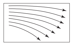
\(\newcommand{\avec}{\mathbf a}\) \(\newcommand{\bvec}{\mathbf b}\) \(\newcommand{\cvec}{\mathbf c}\) \(\newcommand{\dvec}{\mathbf d}\) \(\newcommand{\dtil}{\widetilde{\mathbf d}}\) \(\newcommand{\evec}{\mathbf e}\) \(\newcommand{\fvec}{\mathbf f}\) \(\newcommand{\nvec}{\mathbf n}\) \(\newcommand{\pvec}{\mathbf p}\) \(\newcommand{\qvec}{\mathbf q}\) \(\newcommand{\svec}{\mathbf s}\) \(\newcommand{\tvec}{\mathbf t}\) \(\newcommand{\uvec}{\mathbf u}\) \(\newcommand{\vvec}{\mathbf v}\) \(\newcommand{\wvec}{\mathbf w}\) \(\newcommand{\xvec}{\mathbf x}\) \(\newcommand{\yvec}{\mathbf y}\) \(\newcommand{\zvec}{\mathbf z}\) \(\newcommand{\rvec}{\mathbf r}\) \(\newcommand{\mvec}{\mathbf m}\) \(\newcommand{\zerovec}{\mathbf 0}\) \(\newcommand{\onevec}{\mathbf 1}\) \(\newcommand{\real}{\mathbb R}\) \(\newcommand{\twovec}[2]{\left[\begin{array}{r}#1 \\ #2 \end{array}\right]}\) \(\newcommand{\ctwovec}[2]{\left[\begin{array}{c}#1 \\ #2 \end{array}\right]}\) \(\newcommand{\threevec}[3]{\left[\begin{array}{r}#1 \\ #2 \\ #3 \end{array}\right]}\) \(\newcommand{\cthreevec}[3]{\left[\begin{array}{c}#1 \\ #2 \\ #3 \end{array}\right]}\) \(\newcommand{\fourvec}[4]{\left[\begin{array}{r}#1 \\ #2 \\ #3 \\ #4 \end{array}\right]}\) \(\newcommand{\cfourvec}[4]{\left[\begin{array}{c}#1 \\ #2 \\ #3 \\ #4 \end{array}\right]}\) \(\newcommand{\fivevec}[5]{\left[\begin{array}{r}#1 \\ #2 \\ #3 \\ #4 \\ #5 \\ \end{array}\right]}\) \(\newcommand{\cfivevec}[5]{\left[\begin{array}{c}#1 \\ #2 \\ #3 \\ #4 \\ #5 \\ \end{array}\right]}\) \(\newcommand{\mattwo}[4]{\left[\begin{array}{rr}#1 \amp #2 \\ #3 \amp #4 \\ \end{array}\right]}\) \(\newcommand{\laspan}[1]{\text{Span}\{#1\}}\) \(\newcommand{\bcal}{\cal B}\) \(\newcommand{\ccal}{\cal C}\) \(\newcommand{\scal}{\cal S}\) \(\newcommand{\wcal}{\cal W}\) \(\newcommand{\ecal}{\cal E}\) \(\newcommand{\coords}[2]{\left\{#1\right\}_{#2}}\) \(\newcommand{\gray}[1]{\color{gray}{#1}}\) \(\newcommand{\lgray}[1]{\color{lightgray}{#1}}\) \(\newcommand{\rank}{\operatorname{rank}}\) \(\newcommand{\row}{\text{Row}}\) \(\newcommand{\col}{\text{Col}}\) \(\renewcommand{\row}{\text{Row}}\) \(\newcommand{\nul}{\text{Nul}}\) \(\newcommand{\var}{\text{Var}}\) \(\newcommand{\corr}{\text{corr}}\) \(\newcommand{\len}[1]{\left|#1\right|}\) \(\newcommand{\bbar}{\overline{\bvec}}\) \(\newcommand{\bhat}{\widehat{\bvec}}\) \(\newcommand{\bperp}{\bvec^\perp}\) \(\newcommand{\xhat}{\widehat{\xvec}}\) \(\newcommand{\vhat}{\widehat{\vvec}}\) \(\newcommand{\uhat}{\widehat{\uvec}}\) \(\newcommand{\what}{\widehat{\wvec}}\) \(\newcommand{\Sighat}{\widehat{\Sigma}}\) \(\newcommand{\lt}{<}\) \(\newcommand{\gt}{>}\) \(\newcommand{\amp}{&}\) \(\definecolor{fillinmathshade}{gray}{0.9}\)A set of streamlines for an ideal fluid undergoing steady flow in which there are no sources or sinks for the fluid is shown in Figure 28.3.
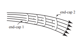
We also show a set of closely separated streamlines that form a flow tube in Figure 28.4 We add to the flow tube two open surface (end-caps 1 and 2) that are perpendicular to velocity of the fluid, of areas \(A_{1}\) and \(A_{2}\), respectively. Because all fluid particles that enter end-cap 1 must follow their respective streamlines, they must all leave end-cap 2. If the streamlines that form the tube are sufficiently close together, we can assume that the velocity of the fluid in the vicinity of each end-cap surfaces is uniform.
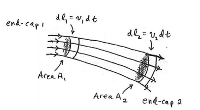
Let \(v_{1}\) denote the speed of the fluid near end-cap 1 and \(v_{2}\) denote the speed of the fluid near end-cap 2. Let \(\rho_{1}\) denote the density of the fluid near end-cap 1 and \(\rho_{2}\) denote the density of the fluid near end-cap 2. The amount of mass that enters and leaves the tube in a time interval \(d t\) can be calculated as follows (Figure 28.5): suppose we consider a small volume of space of cross-sectional area \(A_{2}\) and length \(d l_{1}=v_{1} d t\) near end-cap 1. The mass that enters the tube in time interval \(d t\) is
\[d m_{1}=\rho_{1} d V_{1}=\rho_{1} A_{1} d l_{1}=\rho_{1} A_{1} v_{1} d t \nonumber \]
In a similar fashion, consider a small volume of space of cross-sectional area \(A_{2}\) and length \(d l_{2}=v_{2} d t\) near end-cap 2. The mass that leaves the tube in the time interval dt is then
\[d m_{2}=\rho_{2} d V_{2}=\rho_{2} A_{2} d l_{2}=\rho_{2} A_{2} v_{2} d t \nonumber \]
An equal amount of mass that enters end-cap 1 in the time interval \(d t\) must leave end-cap 2 in the same time interval, thus \(d m_{1}=d m_{2}\). Therefore using Equations (28.3.1) and (28.3.2), we have that \(\rho_{1} A_{1} v_{1} d t=\rho_{2} A_{2} v_{2} d t\). Dividing through by dt implies that
\[\rho_{1} A_{1} v_{1}=\rho_{2} A_{2} v_{2} \quad \text { (steady flow ) } \nonumber \]
Equation (28.3.3) generalizes to any cross sectional area A of the thin tube, where the density is \(\rho\), and the speed is v,
\[\rho A v=\text {constant} \quad \text { (steady flow ) } \nonumber \]
Equation (28.3.3) is referred to as the mass continuity equation for steady flow. If we assume the fluid is incompressible, then Equation (28.3.3) becomes
\[A_{1} v_{1}=A_{2} v_{2}\quad \text { (incompressable fluid, steady flow ) } \nonumber \]
Consider the steady flow of an incompressible with streamlines and closed surface formed by a streamline tube shown in Figure 28.5. According to Equation (28.3.5), when the spacing of the streamlines increases, the speed of the fluid must decrease. Therefore the speed of the fluid is greater entering end-cap 1 then when it is leaving end-cap 2. When we represent fluid flow by streamlines, regions in which the streamlines are widely spaced have lower speeds than regions in which the streamlines are closely spaced.