
17.8: Transverse Oscillations of Masses on a Taut String


- Last updated
- Aug 8, 2022
- Save as PDF

( \newcommand{\kernel}{\mathrm{null}\,}\)
A light string of length 4a is held taut, under tension F between two fixed points.
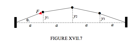
Three equal masses m are attached at equidistant points along the string. They are set into transverse oscillation of small amplitudes, the transverse displacements of the three masses at some time being y1,y2 and y3.
The kinetic energy is easy. It is just
T=12m(˙y21+˙y22+˙y23).
The potential energy is slightly more difficult.
In the undisplaced position, the length of each portion of the string is a.
In the displaced position, the lengths of the four portions of the string are, respectively,
√y2+1+a2√(y2−y1)2+a2√(y2−y3)2+a2√y23+a2
For small displacements (i.e. the ys much smaller than a), these are, approximately (by binomial expansion),
a+y212aa+(y2−y1)22aa+(y2−y3)22aa+y212a
so the extensions are
y212a(y2−y1)22a(y2−y3)22ay232a
It is also supposed that the tension in the string is F and that the displacements are sufficiently small that this is constant. The work done in displacing the masses, which is the elastic energy stored in the string as a result of the displacements, is therefore
V=F2a[y21+(y2−y1)2+(y2−y3)2+y23]=Fa(y21+y22+y23−y1y2−y2y3).
We note with mild irritation the presence of the cross-terms y1y2,y2y3.
Apply Lagrange’s equation in turn to the three coordinates:
am¨y1+F(2y1−y2)=0,
am¨y2+F(−y1+2y2−y3)=0,
am¨y3+F(−y2+2y3)=0.
Seek solutions of the form ¨y1=−ω2y1,¨y2=−ω2y2,¨y2=−ω2y3.
Then
(2F−amω2)y1−Fy2=0,
−Fy1+(2F−amω2)y2−Fy3=0,
−Fy2+(2F−amω2)y3=0.
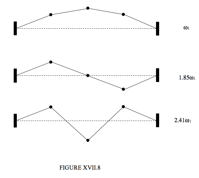
Putting the determinant of the coefficients to zero gives an equation for the frequencies of the normal modes. The solutions are:
| Slow | Medium | Fast |
| ω21=(2−√2Fam | ω22=2Fam | ω23=(2−√2Fam |
Substitution of these into equations ??? to??? gives the following displacement ratios for these three modes:
y1:y2:y3=1:√2:11:0:−11:√2:1
These are illustrated in Figure XVII.8.
As usual, the general motion is a linear combination of the normal modes, the relative amplitudes and phases of the modes depending upon the initial conditions.
If the motion of the first mass is a combination of the three modes with relative amplitudes in the proportion ˆq1:ˆq2:ˆq3 and α1:α2:α3with initial phases its motion is described by
y1=ˆq1sin(ω1t+α1)+ˆq2sin(ω2t+α2)+ˆq3sin(ω3t+α3)
The motions of the second and third masses are then described by
√2ˆq1sin(ω1t+α1)
and
y3=^q1sin(ω1t+α1)−^q2sin(ω2t+α2)+^q3sin(ω3t+α3).
These can be written
y1=q1+q2+q3,
y1=√2q1−√2q3
and
y1=q1−q2+q3,
where the qi, like the yi, are time-dependent coordinates.
We could, if we wish, express the qi in terms of the yi, by solving these equations:
q1=14(y1+√2y2+y3),
q2=12(y1−y3)
and
q3=14(y1−√2y2+y3).
We have hitherto described the state of the system as a function of time by giving the values of the coordinates y1,y2 and y3. We could equally well, if we wished, describe the state of the system by giving, instead, the values of the coordinates q1,q2 and q3. Indeed it turns out that it is very useful to do so, and these coordinates are called the normal coordinates, and we shall see that they have some special properties. Thus, if you express the kinetic and potential energies in terms of the normal coordinates, you get
T=12m(4˙q21+2˙q22+4˙q23)
and
V=2Fa[(2−√2)q21+q22+(2+√2)q23].
Note that there are no cross terms. When you apply Lagrange’s equation in turn to the three normal coordinates, you obtain
am¨q1=−(2−√2)Fq1,
am¨q2=−2Fq2,
and
am¨q3=−(2+√2)Fq3.
Notice that the normal coordinates have become completely separated into three independent equations and that each is of the form ¨q=−ω2q and that each of the normal coordinates oscillates with one of the frequencies of the normal modes. Much of the art of solving problems involving vibrating systems concerns identifying the normal coordinates.