17.5: Double Pendulum

This is another similar problem, though, instead of assuming Hooke’s law, we shall assume that angles are small ( \( \sin \theta \approx \theta , \cos \theta \approx 1 - \frac{1}{2} \theta^2\) ). For clarity of drawing, however, I have drawn large angles in Figure XVIII.4.

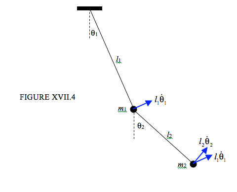
Because I am going to use the lagrangian equations of motion, I have not marked in the forces and accelerations; rather, I have marked in the velocities. I hope that the two components of the velocity of \(m_{2} \) that I have marked are self-explanatory; the speed of \(m_{2} \) is given by \( v^2_{2} = l^2_{1}\dot{\theta}^2_{1} + l^2_{2}\dot{\theta}^2_{2} + 2 l_{1}l_{2}\dot{\theta}_1 \dot{\theta}_2 \cos(\theta_2- \theta_1) \). The kinetic and potential energies are

\[ T = \frac{1}{2}m_1l^2_1\dot{\theta}^2_1 + \frac{1}{2}m_1
[l^2_1\dot{\theta}^2_1 + l^2_2\dot{\theta}^2_2 + 2l_1l_2\dot{\theta}_1\dot{\theta}_2 \cos(\theta_2 - \theta_1)], \label{17.5.1} \]

\[ V = constant - m_1gl_1 \cos \theta_1 - m_2g(l_1\cos \theta_1 + l_2 \cos \theta_2). \label{17.5.2} \]

If we now make the small angle approximation, these become

\[ T = \frac{1}{2} m_1l^2_1 \dot{\theta}^2_1 + \frac{1}{2} m_2(l_1 \dot{\theta}_1 + l_2 \dot{\theta}_2)^2 \label{17.5.3} \]

and

\[ V = contant + \frac{1}{2}m_1gl_1\theta^2_1 + \frac{1}{2}m_1g(l_1\theta^2_1 + l_2\theta^2_2) - m_1gl_1 - m_2gl_2. \label{17.5.4} \]

Apply the lagrangian equation in turn to \( \theta_1\) and \( \theta_2\):

\[ (m_1 + m_2)l^2_1\ddot{\theta}_1 + m_2l_1l_2\ddot{\theta} = -(m_1 + m_2)gl_1 \theta_1 \label{17.5.5} \]

and

\[ m_2l_1l_2 \ddot{\theta}_1 + m_2l^2_2 \ddot{\theta}_2 = -m_2gl_2\theta_2. \label{17.5.6} \]

Seek solutions in the form of \( \dot{\theta}_1 = - \omega \theta_1 \) and \( \dot{\theta}_2 = - \omega^2 \theta_2 \).

Then

\[ (m_1 + m_2)(l_2 \omega^2 -g)\theta_1 + m_2l_1l_2 \omega^2 \theta_2 = 0 \label{17.5.7} \]

and

\[ l_1 \omega^2\theta_1 + (l_2\omega^2 - g)\theta_2 =0. \label{17.5.8} \]

Either of these gives the displacement ratio \( \theta_2/\theta_1 \). Equating the two expressions for the ratio \( \theta_2/\theta_1 \), or putting the determinant of the coefficients to zero, gives the following equation for the frequencies of the normal modes:

\[ m_1l_1l_2\omega^4 - (m_1+m_2)g(l_1+l_2)\omega^2 + (m_1+m_2)g^2 = 0. \label{17.5.9} \]

As in the previous examples, there is a slow in-phase mode, and fast out-of-phase mode.

For example, suppose \(m_1\) = 0.01 kg, \(m_2\) = 0.02 kg, \(l_1 \) = 0.3 m, \(l_2\) = 0.6 m, \(g\) = 9.8 m s⁻².

Then \( 0.0018\omega^4 - 0.02446\omega^2 = 0\). The slow solution is \( \omega \) = 3.441 rad s⁻¹ ( \( P \) = 1.826 s), and the fast solution is \(\omega \) = 11.626 rad s⁻¹ (\(P\) =0.540 s). If we put the first of these (the slow solution) in either of equations 17.5.7 or 8 (or both, as a check against mistakes) we obtain the displacement ratio \( \theta_2 / \theta_1 \) = 1.319, which is an in-phase mode. If we put the second (the fast solution) in either equation, we obtain \( \theta_2 / \theta_1 \) = −0.5689 , which is an out-of-phase mode. If you were to start with\( \theta_2 / \theta_1 \) = 1.319 and let go, the pendulum would swing in the slow in-phase mode. If you were to start with \( \theta_2 / \theta_1 \) = −0.5689 and let go, the pendulum would swing in the fast out-of-phase mode. Otherwise the motion would be a linear combination of the normal modes, with the fraction of each determined by the initial conditions, as in the example in Section 17.3.