
17.10: Water
- Page ID
- 8504

\( \newcommand{\vecs}[1]{\overset { \scriptstyle \rightharpoonup} {\mathbf{#1}} } \)
\( \newcommand{\vecd}[1]{\overset{-\!-\!\rightharpoonup}{\vphantom{a}\smash {#1}}} \)
\( \newcommand{\dsum}{\displaystyle\sum\limits} \)
\( \newcommand{\dint}{\displaystyle\int\limits} \)
\( \newcommand{\dlim}{\displaystyle\lim\limits} \)
\( \newcommand{\id}{\mathrm{id}}\) \( \newcommand{\Span}{\mathrm{span}}\)
( \newcommand{\kernel}{\mathrm{null}\,}\) \( \newcommand{\range}{\mathrm{range}\,}\)
\( \newcommand{\RealPart}{\mathrm{Re}}\) \( \newcommand{\ImaginaryPart}{\mathrm{Im}}\)
\( \newcommand{\Argument}{\mathrm{Arg}}\) \( \newcommand{\norm}[1]{\| #1 \|}\)
\( \newcommand{\inner}[2]{\langle #1, #2 \rangle}\)
\( \newcommand{\Span}{\mathrm{span}}\)
\( \newcommand{\id}{\mathrm{id}}\)
\( \newcommand{\Span}{\mathrm{span}}\)
\( \newcommand{\kernel}{\mathrm{null}\,}\)
\( \newcommand{\range}{\mathrm{range}\,}\)
\( \newcommand{\RealPart}{\mathrm{Re}}\)
\( \newcommand{\ImaginaryPart}{\mathrm{Im}}\)
\( \newcommand{\Argument}{\mathrm{Arg}}\)
\( \newcommand{\norm}[1]{\| #1 \|}\)
\( \newcommand{\inner}[2]{\langle #1, #2 \rangle}\)
\( \newcommand{\Span}{\mathrm{span}}\) \( \newcommand{\AA}{\unicode[.8,0]{x212B}}\)
\( \newcommand{\vectorA}[1]{\vec{#1}} % arrow\)
\( \newcommand{\vectorAt}[1]{\vec{\text{#1}}} % arrow\)
\( \newcommand{\vectorB}[1]{\overset { \scriptstyle \rightharpoonup} {\mathbf{#1}} } \)
\( \newcommand{\vectorC}[1]{\textbf{#1}} \)
\( \newcommand{\vectorD}[1]{\overrightarrow{#1}} \)
\( \newcommand{\vectorDt}[1]{\overrightarrow{\text{#1}}} \)
\( \newcommand{\vectE}[1]{\overset{-\!-\!\rightharpoonup}{\vphantom{a}\smash{\mathbf {#1}}}} \)
\( \newcommand{\vecs}[1]{\overset { \scriptstyle \rightharpoonup} {\mathbf{#1}} } \)
\(\newcommand{\longvect}{\overrightarrow}\)
\( \newcommand{\vecd}[1]{\overset{-\!-\!\rightharpoonup}{\vphantom{a}\smash {#1}}} \)
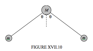
\(\newcommand{\avec}{\mathbf a}\) \(\newcommand{\bvec}{\mathbf b}\) \(\newcommand{\cvec}{\mathbf c}\) \(\newcommand{\dvec}{\mathbf d}\) \(\newcommand{\dtil}{\widetilde{\mathbf d}}\) \(\newcommand{\evec}{\mathbf e}\) \(\newcommand{\fvec}{\mathbf f}\) \(\newcommand{\nvec}{\mathbf n}\) \(\newcommand{\pvec}{\mathbf p}\) \(\newcommand{\qvec}{\mathbf q}\) \(\newcommand{\svec}{\mathbf s}\) \(\newcommand{\tvec}{\mathbf t}\) \(\newcommand{\uvec}{\mathbf u}\) \(\newcommand{\vvec}{\mathbf v}\) \(\newcommand{\wvec}{\mathbf w}\) \(\newcommand{\xvec}{\mathbf x}\) \(\newcommand{\yvec}{\mathbf y}\) \(\newcommand{\zvec}{\mathbf z}\) \(\newcommand{\rvec}{\mathbf r}\) \(\newcommand{\mvec}{\mathbf m}\) \(\newcommand{\zerovec}{\mathbf 0}\) \(\newcommand{\onevec}{\mathbf 1}\) \(\newcommand{\real}{\mathbb R}\) \(\newcommand{\twovec}[2]{\left[\begin{array}{r}#1 \\ #2 \end{array}\right]}\) \(\newcommand{\ctwovec}[2]{\left[\begin{array}{c}#1 \\ #2 \end{array}\right]}\) \(\newcommand{\threevec}[3]{\left[\begin{array}{r}#1 \\ #2 \\ #3 \end{array}\right]}\) \(\newcommand{\cthreevec}[3]{\left[\begin{array}{c}#1 \\ #2 \\ #3 \end{array}\right]}\) \(\newcommand{\fourvec}[4]{\left[\begin{array}{r}#1 \\ #2 \\ #3 \\ #4 \end{array}\right]}\) \(\newcommand{\cfourvec}[4]{\left[\begin{array}{c}#1 \\ #2 \\ #3 \\ #4 \end{array}\right]}\) \(\newcommand{\fivevec}[5]{\left[\begin{array}{r}#1 \\ #2 \\ #3 \\ #4 \\ #5 \\ \end{array}\right]}\) \(\newcommand{\cfivevec}[5]{\left[\begin{array}{c}#1 \\ #2 \\ #3 \\ #4 \\ #5 \\ \end{array}\right]}\) \(\newcommand{\mattwo}[4]{\left[\begin{array}{rr}#1 \amp #2 \\ #3 \amp #4 \\ \end{array}\right]}\) \(\newcommand{\laspan}[1]{\text{Span}\{#1\}}\) \(\newcommand{\bcal}{\cal B}\) \(\newcommand{\ccal}{\cal C}\) \(\newcommand{\scal}{\cal S}\) \(\newcommand{\wcal}{\cal W}\) \(\newcommand{\ecal}{\cal E}\) \(\newcommand{\coords}[2]{\left\{#1\right\}_{#2}}\) \(\newcommand{\gray}[1]{\color{gray}{#1}}\) \(\newcommand{\lgray}[1]{\color{lightgray}{#1}}\) \(\newcommand{\rank}{\operatorname{rank}}\) \(\newcommand{\row}{\text{Row}}\) \(\newcommand{\col}{\text{Col}}\) \(\renewcommand{\row}{\text{Row}}\) \(\newcommand{\nul}{\text{Nul}}\) \(\newcommand{\var}{\text{Var}}\) \(\newcommand{\corr}{\text{corr}}\) \(\newcommand{\len}[1]{\left|#1\right|}\) \(\newcommand{\bbar}{\overline{\bvec}}\) \(\newcommand{\bhat}{\widehat{\bvec}}\) \(\newcommand{\bperp}{\bvec^\perp}\) \(\newcommand{\xhat}{\widehat{\xvec}}\) \(\newcommand{\vhat}{\widehat{\vvec}}\) \(\newcommand{\uhat}{\widehat{\uvec}}\) \(\newcommand{\what}{\widehat{\wvec}}\) \(\newcommand{\Sighat}{\widehat{\Sigma}}\) \(\newcommand{\lt}{<}\) \(\newcommand{\gt}{>}\) \(\newcommand{\amp}{&}\) \(\definecolor{fillinmathshade}{gray}{0.9}\)Water consists of a mass \(M\) (“oxygen”) connected to two smaller equal masses \(m\) (“hydrogen”) by two equal springs of force constants \(k\), the angle between the springs being \(2\theta \). The equilibrium length of each spring is \(r\). The torque needed to increase the angle between the springs by \(2\delta \theta \) is \(2c\delta \theta \). See Figure XVII.10. (\(\theta \) is about 52°.)
At any time, let the coordinates of the three masses (from left to right) be
\( (x_1,y_1), \qquad (x_2,y_2), \qquad (x_3,y_3) \)
and let the equilibrium positions be
\((x_{10},y_{10}), \qquad (x_{20},y_{20}), \qquad (x_{30},y_{30}), \text{ where} y_{30} = y_{10} \)
We suppose that these coordinates are referred to a frame in which the centre of mass of the system is stationary.
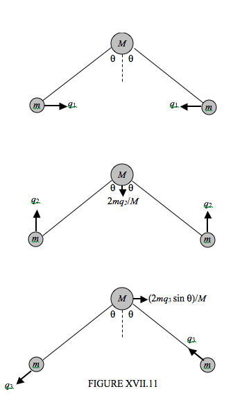
Let us try and imagine, in Figure XVII.11, the vibrational modes. We can easily imagine a mode in which the angle opens and closes symmetrically. Let is resolve this mode into an \(x\)-component and a \(y\)-component. In the \(x\)-component of this motion, one hydrogen atom moves to the right by a distance \(q_1\) while the other moves to the left by and equal distance \(q_1\). In the \(y\)-component of this symmetric motion, both hydrogens move upwards by a distance \(q_2\), while, in order to keep the centre of mass of the system unmoved, the oxygen necessarily moves down by a distance \(2mq_2/M\). We can also imagine an asymmetric mode in which one spring expands while the other contracts. One hydrogen moves down to the left by a distance \(q_3\), while the other moves up to the left by the same distance. In the meantime, the oxygen must move to the right by a distance \((2mq_3 \sin \theta )/M\), in order to keep the centre of mass unmoved.
We are going to try to write down the kinetic and potential energies in terms of the internal coordinates \(q_1, q_2\) and \(q_3\).
It is easy to write down the kinetic energy in terms of the \( (x , y) \) coordinates:
\[ T\ =\ \frac{1}{2}m(\dot{x}_{1}^{2}\ +\ \dot{y}_{1}^{2})\ +\ \frac{1}{2}M(\dot{x}_{2}^{2}\ +\ \dot{y}_{2}^{2})\ +\frac{1}{2}m(\dot{x}_{3}^{2}\ +\ \dot{y}_{3}^{2}). \label{17.10.1} \]
From geometry we have:
\[ \begin{align} \dot{x}_{1} &=\ \dot{q}_{1}-\dot{q}_{3}\sin\theta \\[5pt] \dot{y}_{1} &= \dot{q}_{2}-\dot{q}_{3}\cos\theta \label{17.10.2a,b} \\[5pt] \dot{x}_{2} &= \frac{2m\dot{q}_{3}\sin\theta}{M} \\[5pt] \dot{y}_{2} &= -\frac{2m\dot{q}_{2}}{M} \label{17.10.3a,b} \\[5pt] \dot{x}_{3} &= -\dot{q}_{1} - \dot{q}_{3}\sin\theta \\[5pt] \dot{y}_{3} &= \dot{q}_{2}\ +\ \dot{q}_{3}\cos\theta \label{17.10.4a,b} \end{align} \]
On putting these into equation \( \ref{17.10.1} \) we obtain
\[ T\ =\ m\dot{q}_{1}^{2}\ +\ m\left(1+\frac{2m}{M}\right)\dot{q}_{2}^{2}\ +\ m\left(1+\frac{(2m\sin^{2}\theta)}{M}\right)\dot{q}_{3}^{2} \label{17.10.5} \]
For short, I am going to write this as
\[ T=a_{11}\dot{q}_{1}^{2}+a_{22}\dot{q}_{2}^{2}+a_{33}\dot{q}_{3}^{2} \label{17.10.6} \]
Now for the potential energy.
The extension of the left hand spring is
\[ \delta r_{1}=-q_{1}\sin\theta-q_{2}\cos\theta-\frac{2mq_{2}\cos\theta}{M}+q_{3}+\frac{2mq_{3}\sin\theta\cos\theta}{M}\\=-q_{1}\sin\theta-q_{2}\left(\frac{1+2m}{M}\right)\cos\theta+q_{3}\left(1+\frac{(2m\sin^{2}\theta)}{M }\right) \label{17.10.7} \]
The extension of the right hand spring is
\[ \delta r_{2}=-q_{1}\sin\theta-q_{2}\cos\theta-\frac{2mq_{2}\cos\theta}{M}-q_{3}-\frac{2mq_{3}\sin^{2}\theta}{M}\\=-q_{1}\sin\theta-q_{2}\left(\frac{1+2m}{M}\right)\cos\theta-q_{3}\left(1+\frac{(2m\sin^{2}\theta)}{M }\right). \label{17.10.8} \]
The increase in the angle between the springs is
\[ 2\delta\theta=-\frac{2q_{1}\cos\theta}{r}\ +\ \frac{2(1+\frac{2m}{M})q_{2}\sin\theta}{r}. \label{17.10.9} \]
The potential energy (above the equilibrium position) is
\[ V=\frac{1}{2}k(\delta r_{1})^{2}\ +\ \frac{1}{2}k(\delta r_{2})^{2}\ +\ \frac{1}{2}c(2\delta\theta)^{2}. \label{17.10.10} \]
On substituting Equations \( \ref{17.10.7}\), \( \ref{17.10.8}\) and \( \ref{17.10.9}\) into this, we obtain an equation of the form
\[ V=b_{11}q_{1}^{2}\ +\ 2bq_{12}q_{1}q_{2}\ +\ b_{22}q_{2}^{2}\ +\ b_{33}q_{3}^{2}, \label{17.10.11} \]
where I leave it to the reader, if s/he wishes, to work out the detailed expressions for the coefficients. We still have a cross term, so we can’t completely separate the coordinates, but we can easily apply Lagrange’s equation to Equations \ref{17.10.6} and \ref{17.10.11}, and then seek simple harmonic solutions in the usual way. Setting the determinant of the coefficients to zero leads to the following equation for the angular frequencies of the normal modes:
\[ \begin{bmatrix}b_{11}-\omega^{2}a_{11} & b_{12} & 0 \\ b_{12} & b_{22}-\omega^{2}a_{22} & 0\\ 0 & 0 & b_{33}-\omega^{2}a_{33} \end{bmatrix}\ =\ 0. \label{17.10.12} \]
Thus, given the masses and \(r, \theta, k\) and \(c\), one can predict the frequencies of the normal modes. Can one calculate \(k\) and \(c\) given the frequencies? I do not know, to tell the truth. Can I leave it to the reader to investigate further?