12.2: Worked Examples

Example \(\PageIndex{1}\): Filling a Coal Car

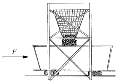
An empty coal car of mass \(m_{0}\) starts from rest under an applied force of magnitude F . At the same time coal begins to run into the car at a steady rate b from a coal hopper at rest along the track (Figure 12.5). Find the speed when a mass \(m_{c}\) of coal has been transferred.

Figure 12.5 Filling a coal car

Solution

We shall analyze the momentum changes in the horizontal direction, which we call the x -direction. Because the falling coal does not have any horizontal velocity, the falling coal is not transferring any momentum in the x -direction to the coal car. So we shall take as our system the empty coal car and a mass \(m_{c}\) of coal that has been transferred. Our initial state at t = 0 is when the coal car is empty and at rest before any coal has been transferred. The x -component of the momentum of this initial state is zero,

\[p_{x}(0)=0 \nonumber \]

Our final state at \(t=t_{f}\) is when all the coal of mass \(m_{c}=b t_{f}\) has been transferred into the car that is now moving at speed \(v_{f}\). The x -component of the momentum of this final state is

\[p_{x}\left(t_{f}\right)=\left(m_{0}+m_{c}\right) v_{f}=\left(m_{0}+b t_{f}\right) v_{f} \nonumber \]

There is an external constant force \(F_{x}=F\) applied through the transfer. The momentum principle applied to the x -direction is

\[\int_{0}^{t_{f}} F_{x} d t=\Delta p_{x}=p_{x}\left(t_{f}\right)-p_{x}(0) \nonumber \]

Because the force is constant, the integral is simple and the momentum principle becomes

\[F t_{f}=\left(m_{0}+b t_{f}\right) v_{f} \nonumber \]

So the final speed is

\[v_{f}=\frac{F t_{f}}{\left(m_{0}+b t_{f}\right)} \nonumber \]

Example \(\PageIndex{2}\): Emptying a Freight Car

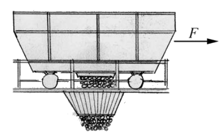
A freight car of mass \(m_{c}\) contains sand of mass \(m_{s}\). At \(t=0\) a constant horizontal force of magnitude F is applied in the direction of rolling and at the same time a port in the bottom is opened to let the sand flow out at the constant rate \(b=d m_{s} / d t\). Find the speed of the freight car when all the sand is gone (Figure 12.6). Assume that the freight car is at rest at \(t=0\).

Figure 12.6 Emptying a freight car

Solution

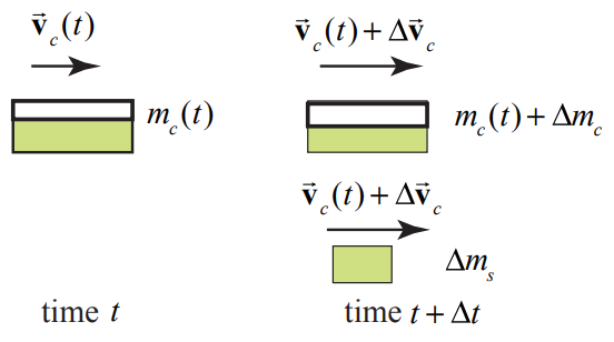
Choose the positive x -direction to point in the direction that the car is moving. Choose for the system the amount of sand in the fright car at time t, \(m_{c}(t)\). At time t , the car is moving with velocity \(\overrightarrow{\mathbf{v}}_{c}(t)=v_{c}(t) \hat{\mathbf{i}}\). The momentum diagram for the system at time t is shown in the diagram on the left in Figure 12.7.

Figure 12.7 Momentum diagram at time t and at time \(t+\Delta t\)

The momentum of the system at time t is given by

\[\overrightarrow{\mathbf{p}}_{s y s}(t)=m_{c}(t) \overrightarrow{\mathbf{v}}_{c}(t) \nonumber \]

During the time interval \([t, t+\Delta t]\), an amount of sand of mass \(\Delta m_{s}\) leaves the freight car and the mass of the freight car changes by \(m_{c}(t+\Delta t)=m_{c}(t)+\Delta m_{c}\), where \(\Delta m_{c}=-\Delta m_{s}\). At the end of the interval the car is moving with velocity \(\overrightarrow{\mathbf{v}}_{c}(t+\Delta t)=\overrightarrow{\mathbf{v}}_{c}(t)+\Delta \overrightarrow{\mathbf{v}}_{c}=\left(v_{c}(t)+\Delta v_{c}\right) \hat{\mathbf{i}}\). The momentum diagram for the system at time \(t+\Delta t\) is shown in the diagram on the right in Figure 12.7. The momentum of the system at time \(t+\Delta t\) is given by

\[\overrightarrow{\mathbf{p}}_{s y s}(t+\Delta t)=\left(\Delta m_{s}+m_{c}(t)+\Delta m_{c}\right)\left(\overrightarrow{\mathbf{v}}_{c}(t)+\Delta \overrightarrow{\mathbf{v}}_{c}\right)=m_{c}(t)\left(\overrightarrow{\mathbf{v}}_{c}(t)+\Delta \overrightarrow{\mathbf{v}}_{c}\right) \nonumber \]

Note that the sand that leaves the car is shown with velocity \(\overrightarrow{\mathbf{v}}_{c}(t)+\Delta \overrightarrow{\mathbf{v}}_{c}\). This implies that all the sand leaves the car with the velocity of the car at the end of the interval. This is an approximation. Because the sand leaves continuous, the velocity will vary from \(\overrightarrow{\mathbf{v}}_{c}(t)\) to \(\overrightarrow{\mathbf{v}}_{c}(t)+\Delta \overrightarrow{\mathbf{v}}_{c}\) but so does the change in mass of the car and these two contributions to the system’s moment exactly cancel. The change in momentum of the system is then

\[\Delta \overrightarrow{\mathbf{p}}_{s y s}=\overrightarrow{\mathbf{p}}_{s y s}(t+\Delta t)-\overrightarrow{\mathbf{p}}_{s y s}(t)=m_{c}(t)\left(\overrightarrow{\mathbf{v}}_{c}(t)+\Delta \overrightarrow{\mathbf{v}}_{c}\right)-m_{c}(t) \overrightarrow{\mathbf{v}}_{c}(t)=m_{c}(t) \Delta \overrightarrow{\mathbf{v}}_{c} \nonumber \]

Throughout the interval a constant force \(\overrightarrow{\mathbf{F}}=F \hat{\mathbf{i}}\) is applied to the system so the momentum principle becomes

\[\overrightarrow{\mathbf{F}}=\lim _{\Delta t \rightarrow 0} \frac{\overrightarrow{\mathbf{p}}_{s y s}(t+\Delta t)-\overrightarrow{\mathbf{p}}_{s y s}(t)}{\Delta t}=\lim _{\Delta t \rightarrow 0} m_{c}(t) \frac{\Delta \overrightarrow{\mathbf{v}}_{c}}{\Delta t}=m_{c}(t) \frac{d \overrightarrow{\mathbf{v}}_{c}}{d t} \nonumber \]

Because the motion is one-dimensional, Equation (12.3.9) written in terms of x -components becomes

\[F=m_{c}(t) \frac{d v_{c}}{d t} \nonumber \]

Denote by initial mass of the car by \(m_{c, 0}=m_{c}+m_{s}\) where \(m_{c}\) is the mass of the car and \(m_{s}\) is the mass of the sand in the car at \(t=0\). The mass of the sand that has left the car at time t is given by

\[m_{s}(t)=\int_{0}^{t} \frac{d m_{s}}{d t} d t=\int_{0}^{t} b d t=b t \nonumber \]

Thus

\[m_{c}(t)=m_{c, 0}-b t=m_{c}+m_{s}-b t \nonumber \]

Therefore Equation (12.3.10) becomes

\[F=\left(m_{c}+m_{s}-b t\right) \frac{d v_{c}}{d t} \nonumber \]

This equation can be solved for the x -component of the velocity at time t , \(v_{c}(t)\) (which in this case is the speed) by the method of separation of variables. Rewrite Equation (12.3.13) as

\[d v_{c}=\frac{F d t}{\left(m_{c}+m_{s}-b t\right)} \nonumber \]

Then integrate both sides of Equation (12.3.14) with the limits as shown

\[\int_{v^{\prime}=0}^{v^{\prime}=v_{c}(t)} d v_{c}^{\prime}=\int_{t^{\prime}=0}^{t^{\prime}=t} \frac{F d t^{\prime}}{m_{c}+m_{s}-b t^{\prime}} \nonumber \]

Integration yields the speed of the car as a function of time

\[v_{c}(t)=-\left.\frac{F}{b} \ln \left(m_{c}+m_{s}-b t^{\prime}\right)\right|_{t=0} ^{\prime^{\prime}=t}=-\frac{F}{b} \ln \left(\frac{m_{c}+m_{s}-b t}{m_{c}+m_{s}}\right)=\frac{F}{b} \ln \left(\frac{m_{c}+m_{s}}{m_{c}+m_{s}-b t}\right) \nonumber \]

In writing Equation (12.3.16), we used the property that \(\ln (a)-\ln (b)=\ln (a / b)\) and therefore \(\ln (a / b)=-\ln (b / a)\). Note that \(m_{c}+m_{s} \geq m_{c}+m_{s}-b t\), so the term \(\ln \left(\frac{m_{c}+m_{s}}{m_{c}+m_{s}-b t}\right) \geq 0\), and the speed of the car increases as we expect.

Example \(\PageIndex{3}\): Filling a Freight Car

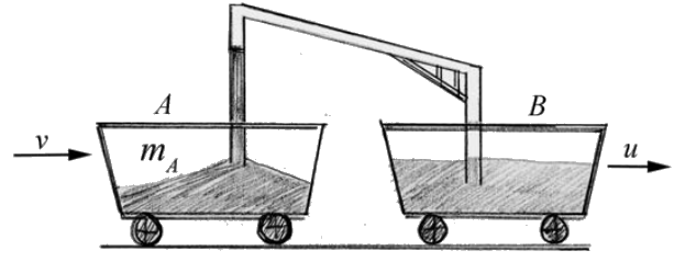
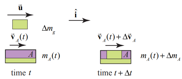
Grain is blown into car A from car B at a rate of b kilograms per second. The grain leaves the chute vertically downward, so that it has the same horizontal velocity, u as car B , (Figure 12.8). Car A is initially at rest before any grain is transferred in and has mass \(m_{A, 0}\). At the moment of interest, car A has mass \(m_{A}\) and speed v . Determine an expression for the speed car A as a function of time t.

Figure 12.8 Filling a freight car

Solution

Choose positive x -direction to the right in the direction the cars are moving. Define the system at time t to be the car and grain that is already in it, which together has mass \(m_{A}(t)\) and the small amount of material of mass \(\Delta m_{g}\) that is blown into car A during the time interval \([t, t+\Delta t]\) At time that is moving with x -component of the velocity \(\mathcal{V}_{A}\). At time t , car A is moving with velocity \(\overrightarrow{\mathbf{v}}_{A}(t)=v_{A}(t) \hat{\mathbf{i}}\) and the material blown into car is moving with velocity \(\overrightarrow{\mathbf{u}}=u \hat{\mathbf{i}}\) At time \(t+\Delta t\) car A is moving with velocity \(\overrightarrow{\mathbf{v}}_{A}(t)+\Delta \overrightarrow{\mathbf{v}}_{A}=\left(v_{A}(t)+\Delta v_{A}\right) \hat{\mathbf{i}}\), and the mass of car A is \(m_{A}(t+\Delta t)=m_{A}(t)+\Delta m_{A}\) where \(\Delta m_{A}=\Delta m_{g}\). The momentum diagram for times t and for \(t+\Delta t\) is shown in Figure 12.9.

Figure 12.9 Momentum diagram at times t and \(t+\Delta t\)

The momentum at time t is

\[\overrightarrow{\mathbf{P}}_{s y s}(t)=m_{A}(t) \overrightarrow{\mathbf{v}}_{A}(t)+\Delta m_{g} \overrightarrow{\mathbf{u}} \nonumber \]

The momentum at time \(t+\Delta t\) is

\[\overrightarrow{\mathbf{P}}_{s y s}(t+\Delta t)=\left(m_{A}(t)+\Delta m_{A}\right)\left(\overrightarrow{\mathbf{v}}_{A}(t)+\Delta \overrightarrow{\mathbf{v}}_{A}\right) \nonumber \]

There are no external forces acting on the system in the x -direction and the external forces acting on the system perpendicular to the motion sum to zero, so the momentum principle becomes

\[\overrightarrow{\mathbf{0}}=\lim _{\Delta t \rightarrow 0} \frac{\overrightarrow{\mathbf{P}}_{s y s}(t+\Delta t)-\overrightarrow{\mathbf{P}}_{s y s}(t)}{\Delta t} \nonumber \]

Using the results above (Equations (12.3.17) and (12.3.18), the momentum principle becomes

\[\overrightarrow{\mathbf{0}}=\lim _{\Delta t \rightarrow 0} \frac{\left(m_{A}(t)+\Delta m_{A}\right)\left(\overrightarrow{\mathbf{v}}_{A}(t)+\Delta \overrightarrow{\mathbf{v}}_{A}\right)-\left(m_{A}(t) \overrightarrow{\mathbf{v}}_{A}(t)+\Delta m_{g} \overrightarrow{\mathbf{u}}\right)}{\Delta t} \nonumber \]

which after using the condition that \(\Delta m_{A}=\Delta m_{g}\) and some rearrangement becomes

\[\overrightarrow{\mathbf{0}}=\lim _{\Delta t \rightarrow 0} \frac{m_{A}(t) \Delta \overrightarrow{\mathbf{v}}_{A}}{\Delta t}+\lim _{\Delta t \rightarrow 0} \frac{\Delta m_{A}\left(\overrightarrow{\mathbf{v}}_{A}(t)-\overrightarrow{\mathbf{u}}\right)}{\Delta t}+\lim _{\Delta t \rightarrow 0} \frac{\Delta m_{A} \Delta \overrightarrow{\mathbf{v}}_{A}}{\Delta t} \nonumber \]

In the limit as , the product \(\Delta m_{A} \Delta \overrightarrow{\mathbf{V}}_{A}\) is a second order differential (the product of two first order differentials) and the term \(\Delta m_{A} \Delta \overrightarrow{\mathbf{v}}_{A} / \Delta t\) approaches zero, therefore the momentum principle yields the differential equation

\[\overrightarrow{\mathbf{0}}=m_{A}(t) \frac{d \overrightarrow{\mathbf{v}}_{A}}{d t}+\frac{d m_{A}}{d t}\left(\overrightarrow{\mathbf{v}}_{A}(t)-\overrightarrow{\mathbf{u}}\right) \nonumber \]

The x -component of Equation (12.3.22) is then

\[0=m_{A}(t) \frac{d v_{A}}{d t}+\frac{d m_{A}}{d t}\left(v_{A}(t)-u\right) \nonumber \]

Rearranging terms and using the fact that the material is blown into car A at a constant rate \(b \equiv d m_{A} / d t\), we have that the rate of change of the x -component of the velocity of car A is given by

\[\frac{d v_{A}(t)}{d t}=\frac{b\left(u-v_{A}(t)\right)}{m_{A}(t)} \nonumber \]

We cannot directly integrate Equation (12.3.24) with respect to dt because the mass of the car A is a function of time. In order to find the x -component of the velocity of car A we need to know the relationship between the mass of car A and the x -component of the velocity of the car A . There are two approaches. In the first approach we separate variables in Equation (12.3.24) where we have suppressed the dependence on t in the expressions for \(m_{A}\) and \(\mathcal{V}_{A}\) yielding

\[\frac{d v_{A}}{u-v_{A}}=\frac{d m_{A}}{m_{A}} \nonumber \]

which becomes the integral equation

\[\int_{v_{A}^{\prime}=0}^{v_{A}^{\prime}=v_{A}(t)} \frac{d v_{A}^{\prime}}{u-v_{A}^{\prime}}=\int_{m_{A}^{\prime}=m_{A, 0}}^{m_{A^{\prime}}^{\prime}=m_{A}(t)} \frac{d m_{A}^{\prime}}{m_{A}^{\prime}} \nonumber \]

where \(m_{A, 0}\) is the mass of the car before any material has been blown in. After integration we have that

\[\ln \frac{u}{u-v_{A}(t)}=\ln \frac{m_{A}(t)}{m_{A, 0}} \nonumber \]

Exponentiate both side yields

\[\frac{u}{u-v_{A}(t)}=\frac{m_{A}(t)}{m_{A, 0}} \nonumber \]

We can solve this equation for the x -component of the velocity of the car

\[v_{A}(t)=\frac{m_{A}(t)-m_{A, 0}}{m_{A}(t)} u \nonumber \]

Because the material is blown into the car at a constant rate \(b \equiv d m_{A} / d t\), the mass of the car as a function of time is given by

\[m_{A}(t)=m_{A, 0}+b t \nonumber \]

Therefore substituting Equation (12.3.30) into Equation (12.3.29) yields the x -component of the velocity of the car as a function of time

\[v_{A}(t)=\frac{b t}{m_{A, 0}+b t} u \nonumber \]

In a second approach, we substitute Equation (12.3.30) into Equation (12.3.24) yielding

\[\frac{d v_{A}}{d t}=\frac{b\left(u-v_{A}\right)}{m_{A, 0}+b t} \nonumber \]

Separate variables in Equation (12.3.32):

\[\frac{d v_{A}}{u-v_{A}}=\frac{b d t}{m_{A, 0}+b t} \nonumber \]

which then becomes the integral equation

\[\int_{v_{A}^{\prime}=0}^{v_{A}^{\prime}=v_{A}(t)} \frac{d v_{A}^{\prime}}{u-v_{A}^{\prime}}=\int_{t^{\prime}=0}^{t^{\prime}=t^{\prime}} \frac{d t^{\prime}}{m_{A, 0}+b t^{\prime}} \nonumber \]

Integration yields

\[\ln \frac{u}{u-v_{A}(t)}=\ln \frac{m_{A, 0}+b t}{m_{A, 0}} \nonumber \]

Again exponentiate both sides resulting in

\[\frac{u}{u-v_{A}(t)}=\frac{m_{A, 0}+b t}{m_{A, 0}} \nonumber \]

After some algebraic manipulation we can find the speed of the car as a function of time

\[v_{A}(t)=\frac{b t}{m_{A, 0}+b t} u \nonumber \]

in agreement with Equation (12.3.31).

Check result:

We can rewrite Equation (12.3.37) as

\[\left(m_{A, 0}+b t\right) v_{A}(t)=b t u \nonumber \]

which illustrates the point that the momentum of the system at time t is equal to the momentum of the grain that has been transferred to the system during the interval [0,t].

Example \(\PageIndex{4}\): Boat and Fire Hose

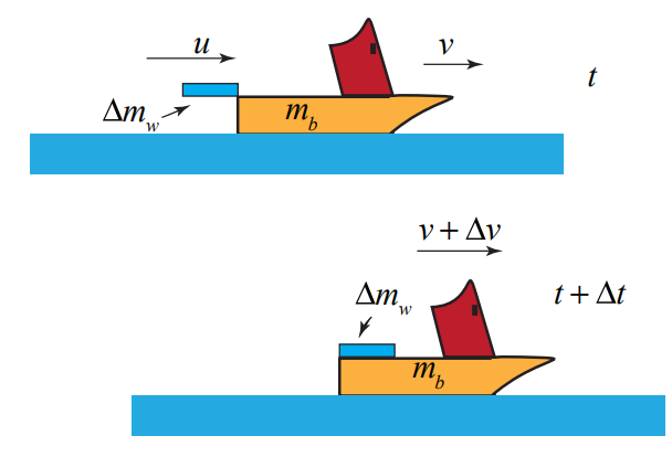
A burning boat of mass \(m_{0}\) is initially at rest. A fire fighter stands on a bridge and sprays water onto the boat. The water leaves the fire hose with a speed u at a rate α (measured in \(\mathrm{kg} \cdot \mathrm{s}^{-1}\)). Assume that the motion of the boat and the water jet are horizontal, that gravity does not play any role, and that the river can be treated as a frictionless surface. Also assume that the change in the mass of the boat is only due to the water jet and that all the water from the jet is added to the boat, (Figure 12.10).

Figure 12.10 Example 12.4

1. In a time interval \([t, t+\Delta t]\), an amount of water \(\Delta m\) hits the boat. Choose a system. Is the total momentum constant in your system? Write down a differential equation that results from the analysis of the momentum changes inside your system.
2. Integrate the differential equation you found in part a), to find the velocity v(m) as a function of the increasing mass m of the boat, \(m_{0}\), and u.

Solution

Let’s take as our system the boat, the amount of water of mass \(\Delta m_{w}\) that enters the boat during the time interval \([t, t+\Delta t]\) and whatever water is in the boat at time t . The water from the fire hose has a speed u . Denote the mass of the boat (including some water) at time t by \(m_{b} \equiv m_{b}(t)\), and the speed of the boat by \(v \equiv v_{b}(t)\). At time \(t+\Delta t\) the speed of the boat is \(v+\Delta v\). Choose the positive x - direction in the direction that the boat is moving. Then the x -components of the momentum of the system at time t and \(t+\Delta t\) are shown in Figure 12.11.

Figure 12.11 Momentum diagrams for burning boat

Because we are assuming that the burning boat slides with negligible resistance and that gravity has a negligible effect on the arc of the water jet, there are no external forces acting on the system in the x -direction. Therefore the x -component of the momentum of the system is constant during the interval \([t, t+\Delta t]\) and so

\[0=\lim _{\Delta t \rightarrow 0} \frac{p_{x}(t+\Delta t)-p_{x}(t)}{\Delta t} \nonumber \]

Using the information from the figure above, Equation (12.3.39) becomes

\[0=\lim _{\Delta t \rightarrow 0} \frac{\left(m_{b}+\Delta m_{w}\right)(v+\Delta v)-\left(\Delta m_{w} u+m_{b} v\right)}{\Delta t} \nonumber \]

Equation (12.3.40) simplifies to

\[0=\lim _{\Delta t \rightarrow 0} m_{b} \frac{\Delta v}{\Delta t}+\lim _{\Delta t \rightarrow 0} \frac{\Delta m_{w}}{\Delta t} v+\lim _{\Delta t \rightarrow 0} \frac{\Delta m_{w} \Delta v}{\Delta t}-\lim _{\Delta t \rightarrow 0} \frac{\Delta m_{w}}{\Delta t} u \nonumber \]

The third term vanishes when we take the limit \(\Delta t \rightarrow 0\) because it is of second order in the infinitesimal quantities (in this case \(\Delta m_{w} \Delta v\)) and when so dividing by \(\Delta t\) the quantity is of first order and hence vanishes since both \(\Delta m_{w} \rightarrow 0\) and \(\Delta v \rightarrow 0\) Equation (12.3.41) becomes

\[0=\lim _{\Delta t \rightarrow 0} m_{b} \frac{\Delta v}{\Delta t}+\lim _{\Delta t \rightarrow 0} \frac{\Delta m_{w}}{\Delta t} v-\lim _{\Delta t \rightarrow 0} \frac{\Delta m_{w}}{\Delta t} u \nonumber \]

We now use the definition of the derivatives:

\[\lim _{\Delta t \rightarrow 0} \frac{\Delta v}{\Delta t}=\frac{d v}{d t} ; \lim _{\Delta t \rightarrow 0} \frac{\Delta m_{w}}{\Delta t}=\frac{d m_{w}}{d t} \nonumber \]

in Equation (12.3.42) to fund the differential equation describing the relation between the acceleration of the boat and the time rate of change of the mass of water entering the boat

\[0=m_{b} \frac{d v}{d t}+\frac{d m_{w}}{d t}(v-u) \nonumber \]

The mass of the boat is increasing due to the addition of the water. Let \(m_{w}(t)\) denote the mass of the water that is in the boat at time t .Then the mass of the boat can be written as

\[m_{b}(t)=m_{0}+m_{w}(t) \nonumber \]

where \(m_{0}\) is the mass of the boat before any water entered. Note we are neglecting the effect of the fire on the mass of the boat. Differentiating Equation (12.3.45) with respect to time yields

\[\frac{d m_{b}}{d t}=\frac{d m_{w}}{d t} \nonumber \]

Then Equation (12.3.44) becomes

\[0=m_{b} \frac{d v}{d t}+\frac{d m_{b}}{d t}(v-u) \nonumber \]

(b) We can integrate this equation through the separation of variable technique. Rewrite Equation (12.3.47) as (cancel the common factor dt )

\[\frac{d v}{v-u}=-\frac{d m_{b}}{m_{b}} \nonumber \]

We can then integrate both sides of Equation (12.3.48) with the limits as shown

\[\int_{v=0}^{v(t)} \frac{d v}{v-u}=-\int_{m_{0}}^{m_{b}(t)} \frac{d m_{b}}{m_{b}} \nonumber \]

Integration yields

\[\ln \left(\frac{v(t)-u}{-u}\right)=-\ln \left(\frac{m_{b}(t)}{m_{0}}\right) \nonumber \]

Recall that \(\ln (a / b)=-\ln (b / a)\) so Equation (12.3.50) becomes

\[\ln \left(\frac{v(t)-u}{-u}\right)=\ln \left(\frac{m_{0}}{m_{b}(t)}\right) \nonumber \]

Also recall that \(\exp (\ln (a / b))=a / b\) and so exponentiating both sides of Equation (12.3.51) yields

\[\frac{v(t)-u}{-u}=\frac{m_{0}}{m_{b}(t)} \nonumber \]

So the speed of the boat at time t can be expressed as

\[v(t)=u\left(1-\frac{m_{0}}{m_{b}(t)}\right) \nonumber \]

Check result:

We can rewrite Equation (12.3.52) as

\[m_{b}(t)(v(t)-u)=-m_{0} u \Rightarrow m_{b}(t) v(t)=\left(m_{b}(t)-m_{0}\right) u \nonumber \]

Recall that the mass of the water that enters the car during the interval [0,t] is \(m_{w}(t)=m_{b}(t)-m_{0}\). Therefore Equation (12.3.54) becomes

\[m_{b}(t) v(t)=m_{w}(t) u \nonumber \]

During the interaction between the jet of water and the boat, the water transfers an amount of momentum \(m_{w}(t) u\) to the boat and car producing a momentum \(m_{b}(t) v(t)\). Because all the water that collides with the boat ends up in the boat, all the interaction forces between the jet of water and the boat are internal forces. The boat recoils forward and the water recoils backward and through collisions with the boat stays in the boat. Therefore if we choose as our system, all of the water that eventually ends up in the boat and the boat then the momentum principle states

\[p_{s y s}(t)=p_{s y s}(0) \nonumber \]

where \(p_{s y s}(0)=m_{w}(t) u\) is the momentum of all of the water that eventually ends up in the boat.

Note that the problem didn’t ask to find the speed of the boat as a function t . We shall now show how to find that. We begin by observing that

\[\frac{d m_{b}}{d t}=\frac{d m_{w}}{d t} \neq \alpha \nonumber \]

where the constant \(\alpha\) is measured in \(\mathrm{kg} \cdot \mathrm{s}^{-1}\) and is specified as a given constant according to the information in the problem statement. The reason is that \(\alpha\) is the rate that the water is ejected from the hose but not the rate that the water enters the boat.

Figure 12.12 Mass per unit length of water jet

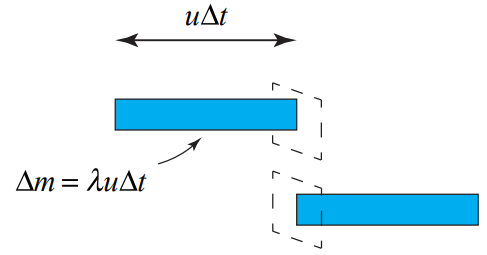
Consider a small amount of water that is moving with speed u that, in a time interval Δt , flows through a cross sectional area oriented perpendicular to the flow (see Figure 12.12). The area is larger than the cross sectional area of the jet of water. The amount of water that floes through the area element \(\Delta m=\lambda u \Delta t\) where λ is the mass per unit length of the jet and \(u \Delta t\) is the length of the jet that flows through the area in the interval Δt . The mass rate of water that flows through the cross sectional area element is then

\[\alpha=\frac{\Delta m}{\Delta t}=\lambda u \nonumber \]

In the Figure 12.13 we consider a small length \(u \Delta t\) of the water jet that is just behind the boat at time t . During the time interval \([t, t+\Delta t]\), the boat moves a distance \(v \Delta t\).

Figure 12.13 Amount of water that enter boat in time interval \([t, t+\Delta t]\)

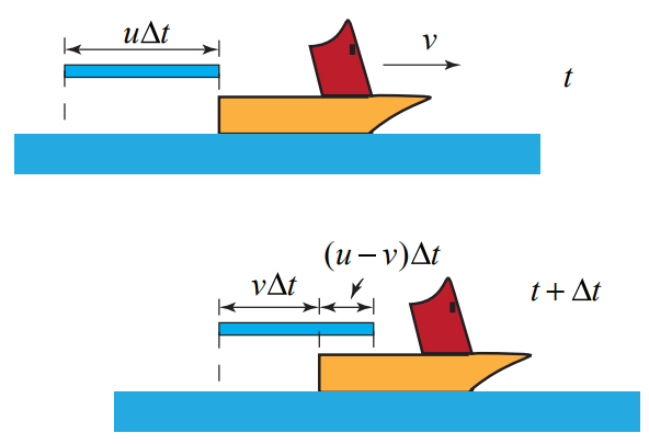
Only a fraction of the length \(u \Delta t\) of water enters the boat and is given by

\[\Delta m_{w}=\lambda(u-v) \Delta t=\frac{\alpha}{u}(u-v) \Delta t \nonumber \]

Dividing Equation (12.3.59) through by \(\Delta t\) and taking limits we have that

\[\frac{d m_{w}}{d t}=\lim _{\Delta t \rightarrow 0} \frac{\Delta m_{w}}{\Delta t}=\frac{\alpha}{u}(u-v)=\alpha\left(1-\frac{v}{u}\right) \nonumber \]

Substituting Equation (12.3.53) and Equation (12.3.46) into Equation (12.3.60) yields

\[\frac{d m_{b}}{d t}=\alpha\left(1-\frac{v}{u}\right)=\alpha \frac{m_{0}}{m_{b}(t)} \nonumber \]

We can integrate this equation by separating variables to find an integral expression for the mass of the boat as a function of time

\[\int_{m_{0}}^{m_{0}(t)} m_{b} d m_{b}=\alpha m_{0} \int_{t=0}^{t} d t \nonumber \]

We can easily integrate both sides of Equation (12.3.62) yielding

\[\frac{1}{2}\left(m_{b}(t)^{2}-m_{0}^{2}\right)=\alpha m_{b, 0} t \nonumber \]

The mass of the boat as a function of time is then

\[m_{b}(t)=m_{0} \sqrt{1+2 \frac{\alpha t}{m_{0}}} \nonumber \]

We now substitute Equation (12.3.64) into Equation (12.3.65)yielding the speed of the burning boat as a function of time

\[v(t)=u\left(1-\frac{1}{\sqrt{1+2 \frac{\alpha t}{m_{b, 0}}}}\right) \nonumber \]