Physics LibreTexts

21.7: Inverse Cube Attractive Force

  • Page ID
    8544
  • \( \newcommand{\vecs}[1]{\overset { \scriptstyle \rightharpoonup} {\mathbf{#1}} } \)

    \( \newcommand{\vecd}[1]{\overset{-\!-\!\rightharpoonup}{\vphantom{a}\smash {#1}}} \)

    \( \newcommand{\id}{\mathrm{id}}\) \( \newcommand{\Span}{\mathrm{span}}\)

    ( \newcommand{\kernel}{\mathrm{null}\,}\) \( \newcommand{\range}{\mathrm{range}\,}\)

    \( \newcommand{\RealPart}{\mathrm{Re}}\) \( \newcommand{\ImaginaryPart}{\mathrm{Im}}\)

    \( \newcommand{\Argument}{\mathrm{Arg}}\) \( \newcommand{\norm}[1]{\| #1 \|}\)

    \( \newcommand{\inner}[2]{\langle #1, #2 \rangle}\)

    \( \newcommand{\Span}{\mathrm{span}}\)

    \( \newcommand{\id}{\mathrm{id}}\)

    \( \newcommand{\Span}{\mathrm{span}}\)

    \( \newcommand{\kernel}{\mathrm{null}\,}\)

    \( \newcommand{\range}{\mathrm{range}\,}\)

    \( \newcommand{\RealPart}{\mathrm{Re}}\)

    \( \newcommand{\ImaginaryPart}{\mathrm{Im}}\)

    \( \newcommand{\Argument}{\mathrm{Arg}}\)

    \( \newcommand{\norm}[1]{\| #1 \|}\)

    \( \newcommand{\inner}[2]{\langle #1, #2 \rangle}\)

    \( \newcommand{\Span}{\mathrm{span}}\) \( \newcommand{\AA}{\unicode[.8,0]{x212B}}\)

    \( \newcommand{\vectorA}[1]{\vec{#1}}      % arrow\)

    \( \newcommand{\vectorAt}[1]{\vec{\text{#1}}}      % arrow\)

    \( \newcommand{\vectorB}[1]{\overset { \scriptstyle \rightharpoonup} {\mathbf{#1}} } \)

    \( \newcommand{\vectorC}[1]{\textbf{#1}} \)

    \( \newcommand{\vectorD}[1]{\overrightarrow{#1}} \)

    \( \newcommand{\vectorDt}[1]{\overrightarrow{\text{#1}}} \)

    \( \newcommand{\vectE}[1]{\overset{-\!-\!\rightharpoonup}{\vphantom{a}\smash{\mathbf {#1}}}} \)

    \( \newcommand{\vecs}[1]{\overset { \scriptstyle \rightharpoonup} {\mathbf{#1}} } \)

    \( \newcommand{\vecd}[1]{\overset{-\!-\!\rightharpoonup}{\vphantom{a}\smash {#1}}} \)

    \(\newcommand{\avec}{\mathbf a}\) \(\newcommand{\bvec}{\mathbf b}\) \(\newcommand{\cvec}{\mathbf c}\) \(\newcommand{\dvec}{\mathbf d}\) \(\newcommand{\dtil}{\widetilde{\mathbf d}}\) \(\newcommand{\evec}{\mathbf e}\) \(\newcommand{\fvec}{\mathbf f}\) \(\newcommand{\nvec}{\mathbf n}\) \(\newcommand{\pvec}{\mathbf p}\) \(\newcommand{\qvec}{\mathbf q}\) \(\newcommand{\svec}{\mathbf s}\) \(\newcommand{\tvec}{\mathbf t}\) \(\newcommand{\uvec}{\mathbf u}\) \(\newcommand{\vvec}{\mathbf v}\) \(\newcommand{\wvec}{\mathbf w}\) \(\newcommand{\xvec}{\mathbf x}\) \(\newcommand{\yvec}{\mathbf y}\) \(\newcommand{\zvec}{\mathbf z}\) \(\newcommand{\rvec}{\mathbf r}\) \(\newcommand{\mvec}{\mathbf m}\) \(\newcommand{\zerovec}{\mathbf 0}\) \(\newcommand{\onevec}{\mathbf 1}\) \(\newcommand{\real}{\mathbb R}\) \(\newcommand{\twovec}[2]{\left[\begin{array}{r}#1 \\ #2 \end{array}\right]}\) \(\newcommand{\ctwovec}[2]{\left[\begin{array}{c}#1 \\ #2 \end{array}\right]}\) \(\newcommand{\threevec}[3]{\left[\begin{array}{r}#1 \\ #2 \\ #3 \end{array}\right]}\) \(\newcommand{\cthreevec}[3]{\left[\begin{array}{c}#1 \\ #2 \\ #3 \end{array}\right]}\) \(\newcommand{\fourvec}[4]{\left[\begin{array}{r}#1 \\ #2 \\ #3 \\ #4 \end{array}\right]}\) \(\newcommand{\cfourvec}[4]{\left[\begin{array}{c}#1 \\ #2 \\ #3 \\ #4 \end{array}\right]}\) \(\newcommand{\fivevec}[5]{\left[\begin{array}{r}#1 \\ #2 \\ #3 \\ #4 \\ #5 \\ \end{array}\right]}\) \(\newcommand{\cfivevec}[5]{\left[\begin{array}{c}#1 \\ #2 \\ #3 \\ #4 \\ #5 \\ \end{array}\right]}\) \(\newcommand{\mattwo}[4]{\left[\begin{array}{rr}#1 \amp #2 \\ #3 \amp #4 \\ \end{array}\right]}\) \(\newcommand{\laspan}[1]{\text{Span}\{#1\}}\) \(\newcommand{\bcal}{\cal B}\) \(\newcommand{\ccal}{\cal C}\) \(\newcommand{\scal}{\cal S}\) \(\newcommand{\wcal}{\cal W}\) \(\newcommand{\ecal}{\cal E}\) \(\newcommand{\coords}[2]{\left\{#1\right\}_{#2}}\) \(\newcommand{\gray}[1]{\color{gray}{#1}}\) \(\newcommand{\lgray}[1]{\color{lightgray}{#1}}\) \(\newcommand{\rank}{\operatorname{rank}}\) \(\newcommand{\row}{\text{Row}}\) \(\newcommand{\col}{\text{Col}}\) \(\renewcommand{\row}{\text{Row}}\) \(\newcommand{\nul}{\text{Nul}}\) \(\newcommand{\var}{\text{Var}}\) \(\newcommand{\corr}{\text{corr}}\) \(\newcommand{\len}[1]{\left|#1\right|}\) \(\newcommand{\bbar}{\overline{\bvec}}\) \(\newcommand{\bhat}{\widehat{\bvec}}\) \(\newcommand{\bperp}{\bvec^\perp}\) \(\newcommand{\xhat}{\widehat{\xvec}}\) \(\newcommand{\vhat}{\widehat{\vvec}}\) \(\newcommand{\uhat}{\widehat{\uvec}}\) \(\newcommand{\what}{\widehat{\wvec}}\) \(\newcommand{\Sighat}{\widehat{\Sigma}}\) \(\newcommand{\lt}{<}\) \(\newcommand{\gt}{>}\) \(\newcommand{\amp}{&}\) \(\definecolor{fillinmathshade}{gray}{0.9}\)

    A particle moves in a field such that the attractive force on it varies inversely as the cube of the distance from a centre of attraction. What is the shape of the path? How does the angle \( \theta \) vary with time?

    Let’s suppose that the radial acceleration is \( a(r) = -k^3/r^3 = - k^3u^3 \). (I want the coefficient of \( 1/r^3\) to be negative, so that the force is attractive, which is why I have written the coefficient as \( -k^2 \). Besides, the dimensions of \(k\) are then L2T−1, which are the same as those of \(h\), the angular momentum per unit mass, which helps to make the algebra simple.) The differential equation to the path (Equation 21.6.10) is then \( h^2 u^2 \frac{d^2u}{d \theta^2} + h^2u^3 = k^2 u^3 \) or

    \[ h^2 \frac{d^2u}{d \theta^2} + h^2u = k^3 u. \label{eq:21.7.11} \]

    That is,

    \[ \frac{d^2u}{d \theta ^2} = \frac{k^2-h^2}{h^2} u. \label{eq:21.7.12} \]

    The form of the motion evidently depends on whether \( k^2 > h^2 \) (a strongly attractive force, or a small angular momentum), or if \( k^2 < h^2 \) (a weak force, or a large angular momentum.) If we start the particle rolling with just the right amount of angular momentum \( ( k^2 = h^2 ) \), there will evidently be zero radial acceleration, and the particle will move in a circle.

    Before integrating Equation \ref{eq:21.7.12}, let us look at the equivalent potential. For \( a(r) = -k^2/r^3 \), the potential in the inertial frame is \( \Omega = -\frac{1}{2} k^2/r^2 \) provided we take the potential at infinity to be zero. The equivalent potential is then (see equation 21.2.5)

    \[ \Omega ' = - \frac{k^2}{2r^2} + \frac{h^2}{2r^2} . \label{eq:21.7.13} \]

    We see that, if \( k^2 = h^2\), the potential is zero and independent of distance. If \( h^2 < k^2\), the equivalent potential is negative, increasing to zero as \(r\) → ∞, and the particle accelerates towards the centre of attraction. If \( h^2 > k^2\), the potential is positive, decreasing to zero as \(r\) → ∞, and the particle accelerates away from the centre of attraction. This sounds like a contradiction, but what is happening is \( h^2 > k^2\), that means that the particle has initially been given a large angular momentum, and, in the corotating frame, the centrifugal force is larger than the attractive force.

    If \( h^2 < k^2\), the equation of motion (Equation \ref{eq:21.7.12}) is

    \[\frac{d^2u}{d \theta^2} = c^2 u , \tag{21.7.14}\label{eq:21.7.14} \]

    where

    \[ c^2 = \frac{k^2 -h^2}{h^2}. \tag{21.7.15}\label{eq:21.7.15} \]

    The general solution is

    \[ u = Ae^{c \theta} + Be^{-c \theta} \tag{21.7.16}\label{eq:21.7.16} \]

    If the initial conditions are that at \(t = 0, r = r_0, u = u_0, \frac{du}{d \theta} = 0 \) (this last condition means that the particle was launched in a direction at right angles to the radius vector, this solution becomes

    \[ u = y_0 \cos h c \theta. \tag{21.7.17}\label{eq:21.7.17} \]

    That is,

    \[ r = r_0 \sec h c \theta\tag{21.7.18}\label{eq:21.7.18} \]

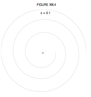
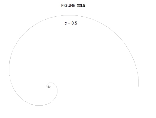
    I have drawn this below for \( c = 0.1 \); that is, for \( k \approx 1.05h \) And for \( c = 0.5 \); that is \( k \approx 1.22h\), for a smaller angular momentum.


    alt

    alt

    We also need to consider the case \( h^2 > k^2 \), in which case the general solution is of the form \(u = A \cos c \theta + B \sin c \theta \). Alas, I haven’t had the energy to do this yet. Perhaps some viewer can beat me to it, and let me know.


    This page titled 21.7: Inverse Cube Attractive Force is shared under a CC BY-NC 4.0 license and was authored, remixed, and/or curated by Jeremy Tatum via source content that was edited to the style and standards of the LibreTexts platform.

    • Was this article helpful?