
1.2: Kinematics- Basic Notions


- Last updated
- Jan 26, 2022
- Save as PDF

( \newcommand{\kernel}{\mathrm{null}\,}\)
The basic notions of kinematics may be defined in various ways, and some mathematicians pay much attention to analyzing such systems of axioms, and relations between them. In physics, we typically stick to less rigorous ways (in order to proceed faster to particular problems) and end debating any definition as soon as "everybody in the room" agrees that we are all speaking about the same thing - at least in the context they are discussed. Let me hope that the following notions used in classical mechanics do satisfy this criterion in our "room":
(i) All the Euclidean geometry notions, including the point, the straight line, the plane, etc.
(ii) Reference frames: platforms for observation and mathematical description of physical phenomena. A reference frame includes a coordinate system used for measuring the point’s position (namely, its radius vector r that connects the coordinate origin to the point - see Figure 1) and a clock that measures time t. A coordinate system may be understood as a certain method of expressing the radius vector r of a point as a set of its scalar coordinates. The most important of such systems (but by no means the only one) are the Cartesian (orthogonal, linear) coordinates 3rj of a point, in which its radius vector may be represented as the following sum: r=3∑j=1njrj, where n1,n2, and n3 are unit vectors directed along the coordinate axis - see Figure 1. 4
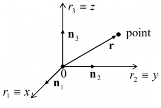 Figure 1.1. Cartesian coordinates of a point
(iii) The absolute ("Newtonian") space/time, 5 which does not depend on the matter distribution. The space is assumed to have the Euclidean metric, which may be expressed as the following relation between the length r of any radius vector r and its Cartesian coordinates: r≡|r|=(3∑j=1r2j)1/2 while time t is assumed to runs similarly in all reference frames.
(iv) The (instant) velocity of the point,
Velocity
v(t)≡drdt≡˙r,
and its acceleration:
Acceleration v(t)≡drdt≡˙ra(t)≡dvdt≡˙v=¨r (v) Transfer between reference frames. The above definitions of vectors r,v, and a depend on the chosen reference frame (are "reference-frame-specific"), and we frequently need to relate those vectors as observed in different frames. Within the Euclidean geometry, the relation between the radius vectors in two frames with the corresponding axes parallel in the moment of interest (Figure 2), is very simple:
Radius transformation
 Figure 1.2. Transfer between two reference frames.
If the frames move versus each other by translation only (no mutual rotation!), similar relations are valid for the velocity and the acceleration as well: v|in 0′=v|in 0+v0|in 0′a|in 0′=a|in 0+a0|in 0′ Note that in the case of mutual rotation of the reference frames, the transfer laws for velocities and accelerations are more complex than those given by Eqs. (6) and (7). Indeed, in this case the notions like v0|in 0′ are not well defined: different points of an imaginary rigid body connected to frame 0 may have different velocities when observed in frame 0 ’. It will be more natural for me to discuss these more general relations in the end of Chapter 4 , devoted to rigid body motion.
(vi) A particle (or "point particle"): a localized physical object whose size is negligible, and the shape is irrelevant for the given problem. Note that the last qualification is extremely important. For example, the size and shape of a spaceship are not too important for the discussion of its orbital motion but are paramount when its landing procedures are being developed. Since classical mechanics neglects the quantum mechanical uncertainties, 6 in it the position of a particle, at any particular instant t, may be identified with a single geometrical point, i.e. with a single radius vector r(t). The formal final goal of classical mechanics is finding the laws of motion r(t) of all particles participating in the given problem.
3 In this series, the Cartesian coordinates (introduced in 1637 by René Descartes, a.k.a. Cartesius) are denoted either as either {r1,r2,r3} or {x,y,z}, depending on convenience in each particular case. Note that axis numbering is important for operations like the vector ("cross") product; the "correct" (meaning generally accepted) numbering order is such that the rotation n1→n2→n3→n1… looks counterclockwise if watched from a point with all rj>0 - like that shown in Figure 1 .
4 Note that the representation (1) is also possible for locally-orthogonal but curvilinear (for example, cylindrical/polar and spherical) coordinates, which will be extensively used in this series. However, such coordinates are not Cartesian, and for them some of the relations given below are invalid - see, e.g., MA Sec. 10 .
5 These notions were formally introduced by Sir Isaac Newton in his main work, the three-volume Philosophiae Naturalis Principia Mathematica published in 1686-1687, but are rooted in earlier ideas by Galileo Galilei, published in 1632.
6 This approximation is legitimate when the product of the coordinate and momentum scales of the particle motion is much larger than Planck’s constant ℏ∼10−34 J⋅s. More detailed conditions of the classical mechanics’ applicability depend on a particular system - see, e.g., the QM part of this series.