7.7: 3D Acoustic Waves

Now moving from the statics to dynamics, we may start with Eq. (24), which may be transformed into the vector form exactly as this was done for the static case in the beginning of Sec. \(4 .\) Comparing Eqs. (24) and (52), we immediately see that the result may be represented as \[\rho \frac{\partial^{2} \mathbf{q}}{\partial t^{2}}=\frac{E}{2(1+v)} \nabla^{2} \mathbf{q}+\frac{E}{2(1+v)(1-2 v)} \nabla(\nabla \cdot \mathbf{q})+\mathbf{f}(\mathbf{r}, t) .\] Let us use this general equation for the analysis of the perhaps most important type of timedependent deformations: acoustic waves. First, let us consider the simplest case of a virtually infinite, uniform elastic medium, with no external forces: \(\mathbf{f}=0\). In this case, due to the linearity and homogeneity of the equation of motion, and taking clues from the analysis of the simple 1D model (see Figure 6.4a) in Secs. 6.3-6.5, \({ }^{33}\) we may look for a particular time-dependent solution in the form of a sinusoidal, linearly-polarized, plane traveling wave \[\mathbf{q}(\mathbf{r}, t)=\operatorname{Re}\left[\mathbf{a} e^{i(\mathbf{k} \cdot \mathbf{r}-\omega t)}\right],\] where \(\mathbf{a}\) is the constant complex amplitude of a wave (now a vector!), and \(\mathbf{k}\) is the wave vector, whose magnitude is equal to the wave number \(k\). The direction of these two vectors should be clearly distinguished: while a determines the wave’s polarization, i.e. the direction of particle displacements, the vector \(\mathbf{k}\) is directed along the spatial gradient of the full phase of the wave \[\Psi \equiv \mathbf{k} \cdot \mathbf{r}-\omega t+\arg a,\] i.e. along the direction of the wave front propagation.

The importance of the angle between these two vectors may be readily seen from the following simple calculation. Let us point the \(z\)-axis of an (inertial) reference frame along the direction of vector \(\mathbf{k}\), and the \(x\)-axis in such direction that the vector \(\mathbf{q}\), and hence a, lie within the \(\{x, z\}\) plane. In this case, all variables may change only along the \(z\)-axis, i.e. \(\nabla=\mathbf{n}_{z}(\partial / \partial z)\), while the amplitude vector may be represented as the sum of just two Cartesian components: \[\mathbf{a}=a_{x} \mathbf{n}_{x}+a_{z} \mathbf{n}_{z} .\] Let us first consider a longitudinal wave, with the particle motion along the wave direction: \(a_{x}=\) \(0, a_{z}=a\). Then the vector \(\mathbf{q}\) in Eq. (107), describing this wave, has only one ( \(z\) ) component, so that \(\nabla \cdot \mathbf{q}\) \(=d q_{z} / d z\) and \(\nabla(\nabla \cdot \mathbf{q})=\mathbf{n}_{z}\left(\partial^{2} \mathbf{q} / \partial z^{2}\right)\), and the Laplace operator gives the same expression: \(\nabla^{2} \mathbf{q}=\) \(\mathbf{n}_{z}\left(\partial^{2} \mathbf{q} / \partial z^{2}\right)\). As a result, Eq. (107), with \(\mathbf{f}=0\), is reduced to a \(1 \mathrm{D}\) wave equation \[\rho \frac{\partial^{2} q_{z}}{\partial t^{2}}=\left[\frac{E}{2(1+v)}+\frac{E}{2(1+v)(1-2 v)}\right] \frac{\partial^{2} q_{z}}{\partial z^{2}} \equiv \frac{E(1-v)}{(1+v)(1-2 v)} \frac{\partial^{2} q_{z}}{\partial z^{2}},\] similar to Eq. (6.40). As we already know from Sec. 6.4, this equation is indeed satisfied with the solution (108), provided that \(\omega\) and \(k\) obey a linear dispersion relation, \(\omega=v_{1} k\), with the following longitudinal wave velocity: \[v_{1}^{2}=\frac{E(1-v)}{(1+v)(1-2 v) \rho} \equiv \frac{K+(4 / 3) \mu}{\rho}\] The last expression allows a simple interpretation. Let us consider a static experiment, similar to the tensile test experiment shown in Figure 6, but with a sample much wider than \(l\) in both directions perpendicular to the force. Then the lateral contraction is impossible \(\left(s_{x x}=s_{y y}=0\right)\), and we can calculate the only finite stress component, \(\sigma_{z z}\), directly from Eq. (34) with \(\operatorname{Tr}(\mathrm{s})=s_{z z}\) : \[\sigma_{z z}=2 \mu\left(s_{z z}-\frac{1}{3} s_{z z}\right)+3 K\left(\frac{1}{3} s_{z z}\right) \equiv\left(K+\frac{4}{3} \mu\right) s_{z z} .\] We see that the numerator in Eq. (112) is nothing more than the static elastic modulus for such a uniaxial deformation, and it is recalculated into the velocity exactly as the spring constant in the 1D waves considered in Secs. 6.3-6.4 - cf. Eq. (6.42).

Formula (114) becomes especially simple in fluids, where \(\mu=0\), and the wave velocity is described by the well-known expression \[v_{1}=\left(\frac{K}{\rho}\right)^{1 / 2}\] Note, however, that for gases, with their high compressibility and temperature sensitivity, the value of \(K\) participating in this formula may differ, at high frequencies, from that given by Eq. (40), because fast compressions/extensions of gas are usually adiabatic rather than isothermal. This difference is noticeable in Table 1 , one of whose columns lists the values of \(v_{l}\) for representative materials.

Now let us consider an opposite case of transverse waves with \(a_{x}=a, a_{z}=0\). In such a wave, the displacement vector is perpendicular to \(\mathbf{n}_{z}\), so that \(\nabla \cdot \mathbf{q}=0\), and the second term on the right-hand side of Eq. (107) vanishes. On the contrary, the Laplace operator acting on such vector still gives the same nonzero contribution, \(\nabla^{2} \mathbf{q}=n_{z}\left(\partial^{2} \mathbf{q} / \partial z^{2}\right)\), to Eq. (107) so that the equation yields \[\rho \frac{\partial^{2} q_{x}}{\partial t^{2}}=\frac{E}{2(1+v)} \frac{\partial^{2} q_{x}}{\partial z^{2}},\] and we again get the linear dispersion relation, \(\omega=v_{t} k\), but with a different velocity:

\[\ \text{Transverse waves: velocity}\quad\quad\quad\quad\nu_{\mathrm{t}}^{2}=\frac{E}{2(1+\nu) \rho}=\frac{\mu}{\rho}.\]

We see that the speed of the transverse waves depends exclusively on the shear modulus \(\mu\) of the medium. \({ }^{34}\) This is also very natural: in such waves, the particle displacements \(\mathbf{q}=\mathbf{n}_{x} q\) are perpendicular to the elastic forces \(d \mathbf{F}=\mathbf{n}_{z} d F\), so that the only one component \(\sigma_{x z}\) of the stress tensor is involved. Also, the strain tensor \(s_{i j}\) ’ has no diagonal components, \(\operatorname{Tr}(\mathrm{s})=0\), so that \(\mu\) is the only elastic modulus actively participating in Hooke’s law (32). In particular, fluids cannot carry transverse waves at all (formally, their velocity (116) vanishes), because they do not resist shear deformations. For all other materials, the longitudinal waves are faster than the transverse ones. \({ }^{35}\) Indeed, for all known natural materials the Poisson ratio is positive so that the velocity ratio that follows from Eqs. (112) and (116), \[\frac{v_{1}}{v_{\mathrm{t}}}=\left(\frac{2-2 v}{1-2 v}\right)^{1 / 2}\] is above \(\sqrt{2} \approx 1.4\). For the most popular construction materials, with \(v \approx 0.3\), the ratio is about \(2-\) see Table \(1 .\)

Let me emphasize again that for both the longitudinal and the transverse waves, the dispersion relation between the wave number and frequency is linear: \(\omega=v k\). As was already discussed in Chapter 6 , in this case of acoustic waves (or just "sound"), the phase and group velocities are equal, and waves of more complex form, consisting of several (or many) Fourier components of the type (108), preserve their form during propagation. This means that both Eqs. (111) and (115) are satisfied by solutions of the type (6.41): \[q_{\pm}(z, t)=f_{\pm}\left(t \mp \frac{z}{v}\right),\] where the functions \(f_{\pm}\)describe the propagating waveforms. (However, if the initial wave is a mixture, of the type (110), of the longitudinal and transverse components, then these components, propagating with different velocities, will "run from each other".) As one may infer from the analysis of a periodic system model in Chapter 6 , the wave dispersion becomes essential at very high (hypersound) frequencies where the wave number \(k\) becomes close to the reciprocal distance \(d\) between the particles of the medium (e.g., atoms or molecules), and hence the approximation of the medium as a continuum, used through this chapter, becomes invalid.

As we already know from Chapter 6, besides the velocity, the waves of each type are characterized by one more important parameter, the wave impedance \(Z\) of the continuum, for acoustic waves frequently called its acoustic impedance. Generalizing Eq. (6.46) to the 3D case, we may define the impedance as the magnitude of the ratio of the force per unit area (i.e. the corresponding component of the stress tensor) exerted by the wave, and the particles’ velocity. For the longitudinal waves, \[Z_{1} \equiv\left|\frac{\sigma_{z z}}{\partial q_{z} / \partial t}\right|=\left|\frac{\sigma_{z z}}{s_{z z}} \frac{s_{z z}}{\partial q_{z} / \partial t}\right|=\left|\frac{\sigma_{z z}}{s_{z z}} \frac{\partial q_{z} / \partial z}{\partial q_{z} / \partial t}\right| \text {. }\] Plugging in Eqs. (108), (112), and (113), we get \[Z_{1}=[(K+4 \mu / 3) \rho]^{1 / 2},\] in a clear analogy with the first of Eqs. (6.48). Similarly, for the transverse waves, the appropriately modified definition, \(Z_{\mathrm{t}} \equiv\left|\sigma_{x z} /\left(\partial q_{x} / \partial z\right)\right|\), yields \[Z_{\mathrm{t}}=(\mu \rho)^{1 / 2}\] Just like in the 1D model studied in Chapter 6, one role of the wave impedance is to scale the power carried by the wave. For plane 3D waves in infinite media, with their infinite wave front area, it is more appropriate to speak about the power density, i.e. power \(/=d \mathscr{P} / d A\) per unit area of the front, and characterize it by not only its magnitude, \[\mu=\frac{d \mathbf{F}}{d A} \cdot \frac{\partial \mathbf{q}}{\partial t},\] but also the direction of the energy propagation, that (for a plane wave in an isotropic medium) coincides with the direction of the wave vector: \(\boldsymbol{h} \equiv / \mathbf{n}_{\mathbf{k}}\). Using the definition (18) of the stress tensor, the Cartesian components of this Umov vector \({ }^{36}\) may be expressed as

\[\mu_{j}=\sum_{j^{\prime}} \sigma_{i j^{\prime}} \frac{\partial q_{j^{\prime}}}{\partial t} .\] Returning to plane waves propagating along axis \(z\), and acting exactly like in Sec. 6 ., for both the longitudinal and transverse waves we again arrive at Eq. (6.49), but for \(/\) rather than \(\mathscr{P}\) (due to a different definition of the wave impedance - per unit area rather than per particle chain). For the sinusoidal waves of the type (108), it yields \[\mu_{z}=\frac{\omega^{2} Z}{2} a a^{*},\] with \(Z\) being the corresponding impedance \(-\) either \(Z_{1}\) or \(Z_{\mathrm{t}}\).

Just as in the 1D case, one more important effect, in which the notion of impedance is crucial, is wave reflection from at an interface between two media. The two boundary conditions, necessary for the analysis of these processes, may be obtained from the continuity of the vectors \(\mathbf{q}\) and \(d \mathbf{F}\). (The former condition is evident, while the latter one may be obtained by applying the \(2^{\text {nd }}\) Newton law to the infinitesimal volume \(d V=d A d z\), where segment \(d z\) straddles the interface.) Let us start from the simplest case of the normal incidence on a plane interface between two uniform media with different elastic moduli and mass densities. Due to the symmetry, it is evident that the longitudinal/transverse incident wave may only excite similarly polarized reflected and transferred waves. As a result, we may literally repeat the calculations of Sec. 6.4, again arriving at the fundamental relations (6.55) and (6.56), with the only replacement of \(Z\) and \(Z^{\prime}\) with the corresponding values of either \(Z_{1}\) (120) or \(Z_{\mathrm{t}}\) (121). Thus, at the normal incidence, the wave reflection is determined solely by the acoustic impedances of the media, while the sound velocities are not involved.

The situation, however, becomes more complicated at a nonzero incidence angle \(\theta^{\text {i) }}\) (Figure 12), where the transmitted wave is generally also refracted, i.e. propagates under a different angle, \(\theta \neq \theta^{(\mathrm{i})}\), beyond the interface. Moreover, at \(\theta^{(\mathrm{i})} \neq 0\) the directions of particle motion (vector \(\mathbf{q}\) ) and of the stress forces (vector \(d \mathbf{F}\) ) in the incident wave are neither exactly parallel nor exactly perpendicular to the interface, and thus this wave serves as an actuator for the reflected and refracted waves of both polarizations - see Figure 12, drawn for the particular case when the incident wave is transverse. The corresponding four angles, \(\theta_{\mathrm{t}}^{(\mathrm{r})}, \theta_{\mathrm{t}}^{(\mathrm{r})}, \theta_{1}^{\prime}, \theta_{\mathrm{t}}^{\prime}\), may be readily related to \(\theta^{(\mathrm{i})}\) by the "kinematic" condition that the incident wave, as well as the reflected and refracted waves of both types, should have the same spatial distribution along the interface plane, i.e. for the interface particles participating in all five waves. According to Eq. (108), the necessary boundary condition is the equality of the tangential components (in Figure \(12, k_{x}\) ), of all five wave vectors: \[k_{\mathrm{t}} \sin \theta_{\mathrm{t}}^{(\mathrm{r})}=k_{1} \sin \theta_{1}^{(\mathrm{r})}=k_{1}^{\prime} \sin \theta_{1}^{\prime}=k_{\mathrm{t}}^{\prime} \sin \theta_{\mathrm{t}}^{\prime}=k_{x} \equiv k_{\mathrm{t}} \sin \theta_{\mathrm{t}}^{(\mathrm{i})} .\] Since the acoustic wave vector magnitudes \(k\), at fixed frequency \(\omega\), are inversely proportional to the corresponding wave velocities, we immediately get the following relations: \[\theta_{\mathrm{t}}^{(\mathrm{r})}=\theta_{\mathrm{t}}^{(\mathrm{i})}, \quad \frac{\sin \theta_{1}^{(\mathrm{r})}}{v_{1}}=\frac{\sin \theta_{1}^{\prime}}{v_{1}^{\prime}}=\frac{\sin \theta_{\mathrm{t}}^{\prime}}{v_{\mathrm{t}}^{\prime}}=\frac{\sin \theta_{\mathrm{t}}^{(\mathrm{i})}}{v_{\mathrm{t}}}\] so that generally all four angles are different. (This is of course an analog of the well-known Snell law in optics - where, however, only transverse waves are possible.) These relations show that, just like in optics, the direction of a wave propagating into a medium with lower velocity is closer to the normal (in Figure 12, the \(z\)-axis). In particular, this means that if \(v^{\prime}>v\), the acoustic waves, at larger angles of incidence, may exhibit the effect of total internal reflection, so well known from optics 37 , when the refracted wave vanishes. In addition, Eqs. (126) show that in acoustics, the reflected longitudinal wave, with velocity \(v_{1}>v_{t}\), may vanish at sufficiently large angles of the transverse wave incidence.

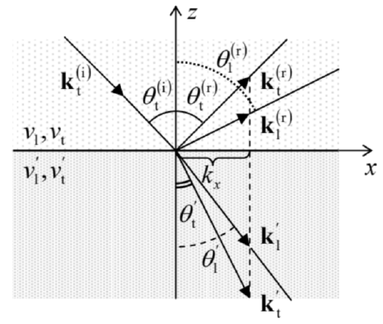Figure 7.12. Deriving the "kinematic" conditions (126) of the acoustic wave reflection and refraction (for the case of a transverse incident wave).

All these facts automatically follow from general expressions for amplitudes of the reflected and refracted waves via the amplitude of the incident wave. These relations are straightforward to derive (again, from the continuity of the vectors \(\mathbf{q}\) and \(d \mathbf{F}\) ), but since they are much bulkier than those in the electromagnetic wave theory (where they are called the Fresnel formulas \({ }^{38}\) ), I would not have time/space to spell out and discuss them. Let me only note that, in contrast to the case of normal incidence, these relations involve eight media parameters: the impedances \(Z, Z^{\prime}\), and the velocities \(v, v^{\prime}\) on both sides of the interface, and for both the longitudinal and transverse waves.

There is another factor that makes boundary acoustic effects more complex. Within certain frequency ranges, interfaces (and in particular surfaces) of elastic solids may sustain so-called surface acoustic waves (SAW), in particular, the Rayleigh waves and the Love waves. \({ }^{39}\) The main feature that distinguishes such waves from their bulk (longitudinal and transverse) counterparts, discussed above, is that the displacement amplitudes are largest at the interface and decay exponentially into the bulk of both adjacent media. The characteristic depth of this penetration is of the order of the wavelength, though not exactly equal to it.

In the Rayleigh waves, the particle displacement vector \(\mathbf{q}\) has two components: one longitudinal (and hence parallel to the interface) and another transverse (perpendicular to the interface). In contrast to the bulk waves, these components are coupled (via their interaction with the interface) and hence propagate with a single velocity \(v_{\mathrm{R}}\). As a result, the trajectory of each particle in the Rayleigh wave is an ellipse in the plane perpendicular to the interface. A straightforward analysis \({ }^{40}\) of the Rayleigh waves on the surface of an elastic solid (i.e. its interface with vacuum) yields the following equation for \(v_{\mathrm{R}}\) : \[\left(2-\frac{v_{\mathrm{R}}^{2}}{v_{\mathrm{t}}^{2}}\right)^{4}=16\left(1-\frac{v_{\mathrm{R}}^{2}}{v_{\mathrm{t}}^{2}}\right)^{2}\left(1-\frac{v_{\mathrm{R}}^{2}}{v_{1}^{2}}\right)^{2} .\] According to this formula, and Eqs. (112) and (116), for realistic materials with the Poisson index between 0 and \(1 / 2\), the Rayleigh waves are slightly (by 4 to \(13 \%\) ) slower than the bulk transverse waves \(-\) and hence substantially slower than the bulk longitudinal waves.

In contrast, the Love waves are purely transverse, with \(\mathbf{q}\) oriented parallel to the interface. However, the interaction of these waves with the interface reduces their velocity \(v_{\mathrm{L}}\) in comparison with that \(\left(v_{\mathrm{t}}\right)\) of the bulk transverse waves, keeping it within the narrow interval between \(v_{\mathrm{t}}\) and \(v_{\mathrm{R}}\) : \[v_{\mathrm{R}}<v_{\mathrm{L}}<v_{\mathrm{t}}<v_{1}\] The practical importance of surface acoustic waves is that their amplitude decays very slowly with distance \(r\) from their point-like source: \(a \propto 1 / r^{1 / 2}\), while any bulk waves decay much faster, as \(a \propto\) \(1 / r\). (Indeed, in the latter case the power \(\mathscr{P} \propto a^{2}\), emitted by such source, is distributed over a spherical surface area proportional to \(r^{2}\), while in the former case all the power goes into a thin surface circle whose length scales as \(r\).) At least two areas of applications of the surface acoustic waves have to be mentioned: in geophysics (for the earthquake detection and the Earth crust seismology), and electronics (for signal processing, with a focus on frequency filtering). Unfortunately, I cannot dwell on these interesting topics and I have to refer the reader to special literature. \({ }^{41}\)

---

\({ }^{33}\) Note though that Eq. (107) is more complex than the simple wave equation (6.40).

\({ }^{34}\) Because of that, one can frequently meet the term shear waves. Note also that in contrast to the transverse waves in the simple 1D model analyzed in Chapter 6 (see Figure 6.4a), those in a 3D continuum do not need a prestretch tension \(\mathscr{T}\). We will return to the effect of tension in the next section.

\({ }^{35}\) Because of this difference between \(v_{1}\) and \(v_{\mathrm{t}}\), in geophysics, the longitudinal waves are known as \(P\)-waves (with the letter P standing for "primary") because they arrive at the detection site, say from an earthquake, first - before the transverse waves, called the \(S\)-waves, with S standing for "secondary".

\({ }^{36}\) Named after Nikolai Alekseevich Umov, who introduced this concept in 1874 - ten years before a similar notion for electromagnetic waves (see, e.g., EM Sec. 6.4) was suggested by J. Poynting. In a dissipation-free, elastic medium, the Umov vector obeys the following continuity equation: \(\partial\left(\rho v^{2} / 2+u\right) / \partial t+\nabla \cdot \boldsymbol{h}=0\), with \(u\) given by Eq. (52), which expresses the conservation of the total (kinetic plus potential) energy of the elastic deformation.

\({ }^{37}\) See, e.g., EM Sec. \(7.5\).

\({ }^{38}\) Their discussion may be also found in EM Sec. \(7.5\).

\({ }^{39}\) Named, respectively, after Lord Rayleigh (born J. Strutt, 1842-1919) who has theoretically predicted the very existence of surface acoustic waves, and A. Love (1863-1940).

\({ }^{40}\) Unfortunately, I do not have time/space to reproduce this calculation either; see, e.g., Sec. 24 in L. Landau and E. Lifshitz, Theory of Elasticity, \(3^{\text {rd }}\) ed., Butterworth-Heinemann, \(1986 .\)

\({ }^{41}\) See, for example, K. Aki and P. Richards, Quantitative Seismology, \(2^{\text {nd }}\) ed., University Science Books, 2002 and D. Morgan, Surface Acoustic Waves, \(2^{\text {nd }}\) ed., Academic Press, \(2007 .\)