7.6: Rod Torsion

One more class of analytically solvable elasticity problems is torsion of quasi-uniform, straight rods by a couple of axially-oriented torques \(\tau=\pm \mathbf{n}_{z} \tau_{z}-\) see Figure 10 .

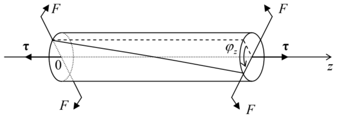Figure 7.10. Rod torsion.

This problem is simpler than the bending in the sense that due to its longitudinal uniformity, \(d \varphi_{z} / d z=\) const, it is sufficient to relate the torque \(\tau_{z}\) to the so-called torsion parameter \[\kappa \equiv \frac{d \varphi_{z}}{d z} .\] If the deformation is elastic and small (in the sense \(\kappa a<<1\), where \(a\) is again the characteristic size of the rod’s cross-section), \(\kappa\) is proportional to \(\tau_{z}\). Hence our task is to calculate their ratio, \[C \equiv \frac{\tau_{z}}{\kappa} \equiv \frac{\tau_{z}}{d \varphi_{z} / d z},\] called the torsional rigidity of the rod.

As the first guess (as we will see below, of a limited validity), one may assume that the torsion does not change either the shape or size of the rod’s cross-sections, but leads just to their mutual rotation about a certain central line. Using a reference frame with the origin on that line, this assumption immediately enables the calculation of Cartesian components of the displacement vector \(d \mathbf{q}\), by using Eq. (6) with \(d \varphi=\mathbf{n}_{z} d \varphi_{z}\) : \[d q_{x}=-y d \varphi_{z}=-\kappa y d z, \quad d q_{y}=x d \varphi_{z}=\kappa x d z, \quad d q_{z}=0 .\] From here, we can calculate all Cartesian components (9) of the symmetrized strain tensor: \[s_{x x}=s_{y y}=s_{z z}=0, \quad s_{x y}=s_{y x}=0, \quad s_{x z}=s_{z x}=-\frac{\kappa}{2} y, \quad s_{y z}=s_{z y}=\frac{\kappa}{2} x .\] The first of these equalities means that the elementary volume does not change, i.e. we are dealing with purely shear deformation. As a result, all nonzero components of the stress tensor, calculated from Eqs. (32), are proportional to the shear modulus alone: \[\sigma_{x x}=\sigma_{y y}=\sigma_{z z}=0, \quad \sigma_{x y}=\sigma_{y x}=0, \quad \sigma_{x z}=\sigma_{z x}=-\mu \kappa y, \quad \sigma_{y z}=\sigma_{z y}=\mu \kappa x .\] (Note that for this problem, with a purely shear deformation, using alternative elastic moduli \(E\) and \(v\) would be rather unnatural. If so desired, we may always use the second of Eqs. (48): \(\mu=E / 2(1+v)\).)

Now it is straightforward to use this result to calculate the full torque as an integral over the cross-section’s area \(A\) : \[\tau_{z} \equiv \int_{A}(\mathbf{r} \times d \mathbf{F})_{z}=\int_{A}\left(x d F_{y}-y d F_{x}\right)=\int_{A}\left(x \sigma_{y z}-y \sigma_{x z}\right) d x d y\] Using Eq. (87), we get \(\tau_{z}=\mu \kappa I_{z}\), i.e. \[C=\mu I_{z}, \text { where } I_{z} \equiv \int_{A}\left(x^{2}+y^{2}\right) d x d y\] Again, just as in the case of thin rod bending, we have got an integral, in this case \(I_{z}\), similar to a moment of inertia, this time for the rotation about the \(z\)-axis passing through a certain point of the crosssection. For any axially-symmetric cross-section, this evidently should be the central point. Then, for example, for the practically important case of a uniform round pipe with internal radius \(R_{1}\) and external radius \(R_{2}\), Eq. (89) yields \[C=\mu 2 \pi \int_{R_{1}}^{R_{2}} \rho^{3} d \rho=\frac{\pi}{2} \mu\left(R_{2}^{4}-R_{1}^{4}\right) .\] In particular, for the solid rod of radius \(R\) (which may be treated as a pipe with \(R_{1}=0\) and \(R_{2}=R\) ), this result gives the following torsional rigidity \[C=\frac{\pi}{2} \mu R^{4},\] while for a hollow pipe of small thickness \(t<<R\), Eq. (90) is reduced to \[C=2 \pi \mu R^{3} t .\] Note that per unit cross-section area \(A\) (and hence per unit mass of the rod) this rigidity is twice higher than that of a solid rod: \[\left.\frac{C}{A}\right|_{\text {thin round pipe }}=\mu R^{2}>\left.\frac{C}{A}\right|_{\text {solid round rod }}=\frac{1}{2} \mu R^{2}\] This fact is one reason for the broad use of thin pipes in engineering and physical experiment design.

However, for rods with axially-asymmetric cross-sections, Eq. (89) gives wrong results. For example, for a narrow rectangle of area \(A=w \times t\) with \(t<<w\), it yields \(C=\mu t w^{3} / 12\) [WRONG!], even functionally different from the correct result - cf. Eq. (104) below. The reason of the failure of the above analysis is that does not describe possible bending \(q_{z}(x, y)\) of the rod’s cross-section in the direction along the rod. (For axially-symmetric rods, such bending is evidently forbidden by the symmetry, so that Eq. (89) is valid, and the results (90)-(92) are absolutely correct.) Let us describe \(^{32}\) this counter-intuitive effect by taking \[q_{z}=\kappa \psi(x, y),\] (where \(\psi\) is some function to be determined), but still keeping Eq. (87) for two other components of the displacement vector. The addition of \(\psi\) does not perturb the equality to zero of the diagonal components of the strain tensor, as well as of \(s_{x y}\) and \(s_{y x}\), but contributes to other off-diagonal components: \[s_{x z}=s_{z x}=\frac{\kappa}{2}\left(-y+\frac{\partial \psi}{\partial x}\right), \quad s_{y z}=s_{z y}=\frac{\kappa}{2}\left(x+\frac{\partial \psi}{\partial y}\right),\] and hence to the corresponding elements of the stress tensor: \[\sigma_{x z}=\sigma_{z x}=\mu \kappa\left(-y+\frac{\partial \psi}{\partial x}\right), \quad \sigma_{y z}=\sigma_{z y}=\mu \kappa\left(x+\frac{\partial \psi}{\partial y}\right) .\] Now let us find the requirement imposed on the function \(\psi(x, y)\) by the fact that the stress force component parallel to the rod’s axis, \[d F_{z}=\sigma_{z x} d A_{x}+\sigma_{z y} d A_{y}=\mu \kappa d A\left[\left(-y+\frac{\partial \psi}{\partial x}\right) \frac{d A_{x}}{d A}+\left(x+\frac{\partial \psi}{\partial y}\right) \frac{d A_{y}}{d A}\right],\] has to vanish at the rod’s surface(s), i.e. at each border of its cross-section. The coordinates \(\{x, y\}\) of any point at a border may be considered as unique functions, \(x(l)\) and \(y(l)\), of the arc \(l\) of that line - see Figure 11 .

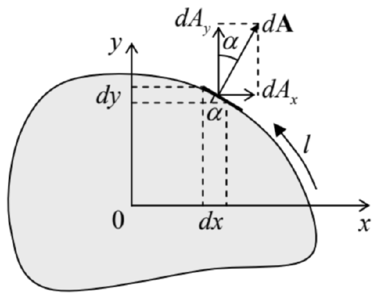
Figure \(7.11\). Deriving Eq. (99).

As this sketch shows, the elementary area ratios participating in Eq. (96) may be readily expressed via the derivatives of these functions: \(d A_{x} / d A=\sin \alpha=d y / d l, d A_{y} / d A=\cos \alpha=-d x / d l\), so that we may write \[\left[\left(-y+\frac{\partial \psi}{\partial x}\right)\left(\frac{d y}{d l}\right)+\left(x+\frac{\partial \psi}{\partial y}\right)\left(-\frac{d x}{d l}\right)\right]_{\mathrm{border}}=0\] Introducing, instead of \(\psi\), a new function \(\chi(x, y)\), defined by its derivatives as

\[\frac{\partial \chi}{\partial x} \equiv \frac{1}{2}\left(-x-\frac{\partial \psi}{\partial y}\right), \quad \frac{\partial \chi}{\partial y} \equiv \frac{1}{2}\left(-y+\frac{\partial \psi}{\partial x}\right)\] we may rewrite Eq. (97) as \[\left.2\left(\frac{\partial \chi}{\partial y} \frac{d y}{d l}+\frac{\partial \chi}{\partial x} \frac{d x}{d l}\right)_{\text {border }} \equiv 2 \frac{d \chi}{d l}\right|_{\text {border }}=0,\] so that the function \(\chi\) should be constant at each border of the cross-section.

In particular, for a singly-connected cross-section, limited by just one continuous border line (as in Figure 11), this constant is arbitrary, because according to Eqs. (98), its choice does not affect the longitudinal deformation function \(\psi(x, y)\) and hence the deformation as the whole. Now let use the definition (98) of the function \(\chi\) to calculate the 2D Laplace operator of this function: \[\nabla_{x, y}^{2} \chi \equiv \frac{\partial^{2} \chi}{\partial^{2} x}+\frac{\partial^{2} \chi}{\partial^{2} y}=\frac{1}{2} \frac{\partial}{\partial x}\left(-x-\frac{\partial \psi}{\partial y}\right)+\frac{1}{2} \frac{\partial}{\partial y}\left(-y+\frac{\partial \psi}{\partial y}\right) \equiv-1 .\] This a 2D Poisson equation (frequently met, for example, in electrostatics), but with a very simple, constant right-hand side. Plugging Eqs. (98) into Eqs. (95), and those into Eq. (88), we may express the torque \(\tau\), and hence the torsional rigidity \(C\), via the same function: \[C \equiv \frac{\tau_{z}}{\kappa}=-2 \mu \int_{A}\left(x \frac{\partial \chi}{\partial x}+y \frac{\partial \chi}{\partial y}\right) d x d y .\] Sometimes, it is easier to use this result in either of its two different forms. The first of them may be readily obtained from Eq. (101a) using integration by parts: \[\begin{aligned} C &=-2 \mu\left(\int d y \int x d \chi+\int d x \int y d \chi\right)=-2 \mu\left[\int d y\left(x \chi_{\text {border }}-\int \chi d x\right)+\int d x\left(y \chi_{\text {border }}-\int \chi d y\right)\right] \\ &=4 \mu\left[\int_{A} \chi d x d y-\chi_{\text {border }} \int d x d y\right], \end{aligned}\] while the proof of one more form, \[C=4 \mu \int_{A}\left(\nabla_{x, y} \chi\right)^{2} d x d y\] is left for the reader’s exercise.

Thus, if we need to know the rod’s rigidity alone, it is sufficient to calculate the function \(\chi(x, y)\) from Eq. (100) with the boundary condition \(\left.\chi\right|_{\text {border }}=\) const, and then plug it into any of Eqs. (101). Only if we are also curious about the longitudinal deformation (93) of the cross-section, we may continue by using Eq. (98) to find the function \(\psi(x, y)\) describing this deformation. Let us see how does this general result work for the two examples discussed above. For the round cross-section of radius \(R\), both the Poisson equation (100) and the boundary condition, \(\chi=\) const at \(x^{2}+y^{2}=R^{2}\), are evidently satisfied by the axially-symmetric function \[\chi=-\frac{1}{4}\left(x^{2}+y^{2}\right)+\text { const. }\] For this case, either of Eqs. (101) yields \[C=4 \mu \int_{A}\left[\left(-\frac{1}{2} x\right)^{2}+\left(-\frac{1}{2} y\right)^{2}\right] d x d y=\mu \int_{A}\left(x^{2}+y^{2}\right) d^{2} r,\] i.e. the same result (89) that we had for \(\psi=0\). Indeed, plugging Eq. (102) into Eqs. (98), we see that in this case \(\partial \psi / \partial x=\partial \psi / \partial y=0\), so that \(\psi(x, y)=\) const, i.e. the cross-section is not bent. (As was discussed in Sec. 1, a uniform translation \(d q_{z}=\kappa \psi=\) const does not constitute a deformation. )

Now, turning to a rod with a narrow rectangular cross-section \(A=w \times t\) with \(t<<w\), we may use this strong inequality to solve the Poisson equation (100) approximately, neglecting the second derivative of \(\chi\) along the wider dimension (say, \(y\) ). The remaining 1D differential equation \(d^{2} \chi / d^{2} x=-1\), with boundary conditions \(\left.\chi\right|_{x=+t / 2}=\left.\chi\right|_{x=-t / 2}\) has an evident solution: \(\chi=-x^{2} / 2+\) const. Plugging this expression into any form of Eq. (101), we get the following (correct) result for the torsional rigidity: \[C=\frac{1}{6} \mu w t^{3} \text {. }\] Now let us have a look at the cross-section bending law (93) for this particular case. Using Eqs. (96), we get \[\frac{\partial \psi}{\partial y}=-x-2 \frac{\partial \chi}{\partial x}=x, \quad \frac{\partial \psi}{\partial x}=y+2 \frac{\partial \chi}{\partial y}=y .\] Integrating these differential equations over the cross-section, and taking the integration constant (again, not contributing to the deformation) for zero, we get a beautifully simple result: \[\psi=x y, \quad \text { i.e. } q_{z}=\kappa x y .\] It means that the longitudinal deformation of the rod has a "propeller bending" form: while the regions near the opposite corners (on the same diagonal) of the cross-section bend toward one direction of the \(z\) axis, the corners on the other diagonal bend in the opposite direction. (This qualitative conclusion remains valid for rectangular cross-sections with any "aspect ratio" \(t / w\).)

For rods with several surfaces, i.e. with cross-sections limited by several boundaries (say, hollow pipes), finding the function \(\chi(x, y)\) requires a bit more care, and Eq. (103b) has to be modified, because it may be equal to a different constant at each boundary. Let me leave the calculation of the torsional rigidity for this case for the reader’s exercise.

---

\({ }^{32}\) I would not be terribly shocked if the reader skipped the balance of this section at the first reading. Though the calculation described in it is very elegant, instructive, and typical for the advanced theory of elasticity, its results will not be used in other chapters of this course or other parts of this series.