7.8: Elastic Waves in Thin Rods

From what we have discussed at the end of the last section, it should be pretty clear that generally, the propagation of acoustic waves in elastic bodies of finite size may be very complicated. There is, however, one important limit in which several important results may be readily obtained. This is the limit of (relatively) low frequencies, where the corresponding wavelength is much larger than at least one dimension of a system. Let us consider, for example, various waves that may propagate along thin rods, in this case "thin" meaning that the characteristic size \(a\) of the rod’s cross-section is much smaller than not only the length of the rod, but also the wavelength \(\lambda=2 \pi / k\). In this case, there is a considerable range of distances \(z\) along the rod, \[a<<\Delta z<<\lambda,\] in that we can neglect the material’s inertia, and apply the results of our earlier static analyses.

For example, for a longitudinal wave of stress, which is essentially a wave of periodic tensile extensions and compressions of the rod, within the range (129) we may use the static relation (42):

\[\sigma_{z z}=E s_{z z} .\] For what follows, it is easier to use the general equation of elastic dynamics not in its vector form (107), but rather in the precursor, Cartesian-component form \((25)\), with \(f_{j}=0\). For plane waves propagating along the \(z\)-axis, only one component (with \(j^{\prime} \rightarrow z\) ) of the sum on the right-hand side of this equation is not equal to zero, and it is reduced to \[\rho \frac{\partial^{2} q_{j}}{\partial^{2} t^{2}}=\frac{\partial \sigma_{j z}}{\partial z} .\] In our current case of longitudinal waves, all components of the stress tensor but \(\sigma_{z z}\) are equal to zero. With \(\sigma_{z z}\) from Eq. (130), and using the definition \(s_{z z}=\partial q_{z} / \partial z\), Eq. (131) is reduced to a simple wave equation, \[\rho \frac{\partial^{2} q_{z}}{\partial^{2} t^{2}}=E \frac{\partial^{2} q_{z}}{\partial z^{2}},\] which shows that the velocity of such tensile waves is \[v=\left(\frac{E}{\rho}\right)^{1 / 2}\] Comparing this result with Eq. (112), we see that the tensile wave velocity, for any realistic material with a positive Poisson ratio, is lower than the velocity \(v_{1}\) of longitudinal waves in the bulk of the same material. The reason for this difference is simple: in thin rods, the cross-section is free to oscillate (e.g., shrink in the longitudinal extension phase of the passing wave), \({ }^{42}\) so that the effective force resisting the longitudinal deformation is smaller than in a border-free space. Since (as it is clearly visible from the wave equation), the scale of the force determines that of \(v^{2}\), this difference translates into slower waves in rods. Of course, as the wave frequency is increased to \(k a \sim 1\), there is a (rather complex and cross-section-depending) crossover from Eq. (133) to Eq. (112).

Proceeding to transverse waves in rods, let us first have a look at long bending waves, for which the condition (129) is satisfied, so that the vector \(\mathbf{q}=\mathbf{n}_{x} q_{x}\) (with the \(x\)-axis being the bending direction see Figure 8) is virtually constant in the whole cross-section. In this case, the only component of the stress tensor contributing to the net transverse force \(F_{x}\) is \(\sigma_{x z}\), so that the integral of Eq. (131) over the crosssection is \[\rho A \frac{\partial^{2} q_{x}}{\partial t^{2}}=\frac{\partial F_{x}}{\partial z}, \quad \text { with } F_{x}=\int_{A} \sigma_{x z} d^{2} r .\] Now, if Eq. (129) is satisfied, we again may use the static local relations (75)-(77), with all derivatives \(d / d z\) duly replaced with their partial form \(\partial / \partial z\), to express the force \(F_{x}\) via the bending deformation \(q_{x}\). Plugging these relations into each other one by one, we arrive at a rather unusual differential equation \[\rho A \frac{\partial^{2} q_{x}}{\partial t^{2}}=-E I_{y} \frac{\partial^{4} q_{x}}{\partial z^{4}} .\] Looking for its solution in the form of a sinusoidal wave (108), we get the following nonlinear dispersion relation: 43 \[\omega=\left(\frac{E I_{y}}{\rho A}\right)^{1 / 2} k^{2} .\] Such relation means that the bending waves are not acoustic at any frequency, and cannot be characterized by a single velocity that would be valid for all wave numbers \(k\), i.e. for all spatial Fourier components of a waveform. According to our discussion in Sec. 6.3, such strongly dispersive systems cannot pass non-sinusoidal waveforms too far without changing their waveform rather considerably.

This situation changes, however, if the rod is pre-stretched with a tension force \(\mathscr{T}\) - just as in the discrete 1D model that was analyzed in Sec. 6.3. The calculation of the effect of this force is essentially similar; let us repeat it for the continuous case, for a minute neglecting the bending stress - see Figure \(13 .\)

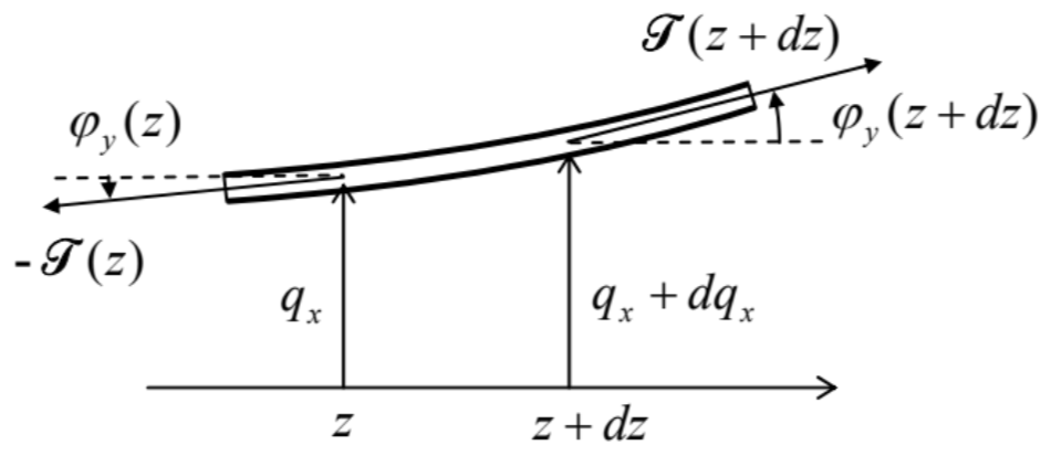
Fig. 7.13. Additional forces in a thin rod (“string”), due to the background tension \(\ \mathscr{T}\).

Still sticking to the limit of small angles \(\varphi\), the additional vertical component \(d \mathscr{T}_{x}\) of the net force acting on a small rod fragment of length \(d z\) is \(\mathscr{T}_{x}(z-d z)-\mathscr{T}_{x}(z)=\mathscr{T} \varphi_{y}(z+d z)-\mathscr{T} \varphi_{y}(z) \approx \mathscr{T}\left(\partial \varphi_{y} / \partial z\right) d z\), so that \(\partial F_{x} / \partial z=\mathscr{T}\left(\partial \varphi_{y} / \partial z\right)\). With the geometric relation (77) in its partial-derivative form \(\partial q_{x} / \partial z=\varphi_{y}\), this additional term becomes \(\mathcal{T}\left(\partial^{2} q_{x} / \partial z^{2}\right)\). Now adding it to the right-hand side of Eq. (135), we get the following dispersion relation \[\omega^{2}=\frac{1}{\rho A}\left(E I_{y} k^{4}+\mathscr{T}^{2}\right)\] Since the product \(\rho A\) in the denominator of this expression is just the rod’s mass per unit length (which was denoted \(\mu\) in Chapter 6), at low \(k\) (and hence low frequencies), this expression is reduced to the linear dispersion law, with the velocity given by Eq. (6.43): \[v=\left(\frac{\mathscr{T}}{\rho A}\right)^{1 / 2} .\] So Eq. (137) describes a smooth crossover from the "guitar-string" acoustic waves to the highly dispersive bending waves (136).

Now let us consider another type of transverse waves in thin rods - the so-called torsional waves, which are essentially the dynamic propagation of the torsional deformation discussed in Sec. 6 . The easiest way to describe these waves, again within the limits (129), is to write the equation of rotation of a small segment \(d z\) of the rod about the \(z\)-axis, passing through the "center of mass" of its cross-section, under the difference of torques \(\tau=\mathbf{n}_{z} \tau_{z}\) applied on its ends - see Figure 10: \[\rho I_{z} d z \frac{\partial^{2} \varphi_{z}}{\partial t^{2}}=d \tau_{z},\] where \(I_{z}\) is the "moment of inertia" defined by Eq. (91), which now, after its multiplication by \(\rho d z\), i.e. by the mass per unit area, has turned into the genuine moment of inertia of a \(d z\)-thick slice of the rod. Dividing both sides of Eq. (139) by \(d z\), and using the static local relation (84), \(\tau_{z}=C \kappa=C\left(\partial \varphi_{z} / \partial z\right)\), we get the following differential equation \[\rho I_{z} \frac{\partial^{2} \varphi_{z}}{\partial t^{2}}=C \frac{\partial^{2} \varphi_{z}}{\partial z^{2}} .\] Just as Eqs. (111), (115), and (132), this equation describes an acoustic (dispersion-free) wave, which propagates with the following frequency-independent velocity \[v=\left(\frac{C}{\rho I_{z}}\right)^{1 / 2} .\] As we have seen in Sec. 6, for rods with axially-symmetric cross-sections, the torsional rigidity \(C\) is described by the simple relation (89), \(C=\mu I_{z}\), so that Eq. (141) is reduced to Eq. (116) for the transverse waves in infinite media. The reason for this similarity is simple: in a torsional wave, particles oscillate along small arcs (Figure 14a), so that if the rod’s cross-section is round, its surface is stress-free, and does not perturb or modify the motion in any way, and hence does not affect the transverse velocity.

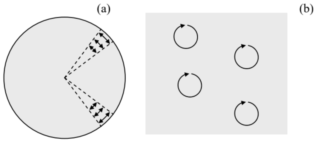Figure 7.14. Particle trajectories in two different transverse waves with the same velocity: (a) torsional waves in a thin round rod and (b) circularly-polarized waves in an infinite (or very broad) sample.

This fact raises an interesting issue of the relation between the torsional and circularly-polarized waves. Indeed, in Sec. 7, I have not emphasized enough that Eq. (116) is valid for a transverse wave polarized in any direction perpendicular to vector \(\mathbf{k}\) (in our notation, directed along the \(z\)-axis). In particular, this means that such waves are doubly-degenerate: any isotropic elastic continuum can carry simultaneously two non-interacting transverse waves propagating in the same direction with the same velocity (116), with two mutually perpendicular linear polarizations (directions of the vector a), for example, directed along the \(x\) - and \(y\)-axes. \({ }^{44}\) If both waves are sinusoidal (108), with the same frequency, each point of the medium participates in two simultaneous sinusoidal motions within the \([x, y]\) plane: \[q_{x}=\operatorname{Re}\left[a_{x} e^{i(k z-\omega t)}\right]=A_{x} \cos \Psi, \quad q_{y}=\operatorname{Re}\left[a_{y} e^{i(k z-\omega t)}\right]=A_{y} \cos (\Psi+\varphi),\] where \(\Psi \equiv k z-\omega t+\varphi_{x}\), and \(\varphi \equiv \varphi_{y}-\varphi_{x}\). Basic geometry tells us that the trajectory of such a motion on the \([x, y]\) plane is an ellipse (Figure 15), so that such waves are called elliptically polarized. The most important particular cases of such polarization are:

(i) \(\varphi=0\) or \(\pi\). a linearly-polarized wave, with vector a is directed at angle \(\theta=\tan ^{-1}\left(A_{y} / A_{x}\right)\) relatively the axis \(x\); and

(ii) \(\varphi=\pm \pi / 2\) and \(A_{x}=A_{y}\) : two possible circularly-polarized waves, with the right or left polarization, respectively. \({ }_{4}^{4}\)

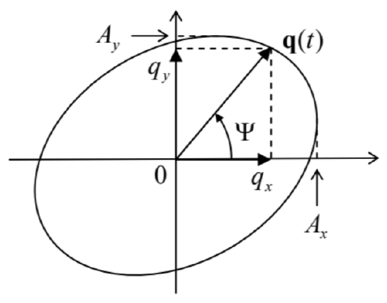Figure 7.15. The trajectory of a particle in an elliptically polarized transverse wave, within the plane perpendicular to the direction of wave propagation.

Now comparing the trajectories of particles in the torsional wave in a thin round rod (or pipe) and the circularly-polarized wave in a broad sample (Figure 14), we see that, despite the same wave propagation velocity, these transverse waves are rather different. In the former case (Figure 14a) each particle moves back and forth along an arc, with the arc length different for different particles (and vanishing at the rod’s center), so that the waves are not plane. On the other hand, in a circularly polarized wave, all particles move along similar, circular trajectories, so that such wave \(i s\) plane.

To conclude this chapter, let me briefly mention the opposite limit, when the size of the body, from whose boundary the waves are completely reflected, \({ }^{46}\) is much larger than the wavelength. In this case, the waves propagate almost as in an infinite 3D continuum (which was analyzed in Sec. 7), and the most important new effect is the finite numbers of wave modes in the body. Repeating the \(1 \mathrm{D}\) analysis at the end of Sec. 6.5, for each dimension of a 3D cuboid of volume \(V=l_{1} l_{2} l_{3}\), and taking into account that the numbers \(k_{n}\) in each of 3 dimensions are independent, we get the following generalization of Eq. (6.75) for the number \(\Delta N\) of different traveling waves with wave vectors within a relatively small volume \(d^{3} k\) of the wave vector space: \[d N=g \frac{V}{(2 \pi)^{3}} d^{3} k \gg 1, \quad \text { for } \frac{1}{V}<<d^{3} k<<k^{3},\] where \(k \gg>>1 / l_{1,2,3}\) is the center of this volume, and \(g\) is the number of different possible wave modes with the same wave vector \(\mathbf{k}\). For the mechanical waves analyzed above, with one longitudinal mode, and two transverse modes with different polarizations, \(g=3\).

Note that since the derivation of Eqs. (6.75) and (143) does not use other properties of the waves (in particular, their dispersion relations), the mode counting rule is ubiquitous in physics, being valid, in particular, for electromagnetic waves (where \(g=2\) ) and quantum "de Broglie waves" (i.e. wavefunctions), whose degeneracy factor \(g\) is usually determined by the particle’s spin. \({ }^{47}\)

---

\({ }^{42}\) For this reason, the tensile waves can be called longitudinal only in a limited sense: while the stress wave is purely longitudinal: \(\sigma_{x x}=\sigma_{y y}=0\), the strain wave is not: \(s_{x x}=s_{y y}=-\sigma_{z z} \neq 0\), i.e. \(\mathbf{q}(\mathbf{r}, t) \neq \mathbf{n}_{z} q_{z}\).

\({ }^{43}\) Note that since the "moment of inertia" \(I_{y}\), defined by Eq. (70), may depend on the bending direction (unless the cross-section is sufficiently symmetric), the dispersion relation (136) may give different results for different directions of the bending wave polarization.

\({ }^{44}\) As was shown in Sec. 6.3, this is true even in the simple 1D model shown in Figure 6.4a.

\({ }^{45}\) The circularly polarized waves play an important role in quantum mechanics, where they may be most naturally quantized, with their elementary excitations (in the case of mechanical waves we are discussing, called phonons) having either positive or negative angular momentum \(L_{z}=\pm \hbar\).

\({ }^{46}\) For acoustic waves, such a condition is easy to implement. Indeed, from Sec. 7 we already know that the strong inequality of wave impedances \(Z\) is sufficient for such reflection. The numbers of Table 1 show that, for example, the impedance of a longitudinal wave in a typical metal (say, steel) is almost two orders of magnitude higher than that in air, ensuring their virtually full reflection from the surface.

\({ }^{47}\) See, e.g., EM Secs. \(7.8\) and QM Sec. 1.7.