2.10: Lagrange Multipliers

The problem of finding minima (or maxima) of a function subject to constraints was first solved by Lagrange. A simple example will suffice to show the method.

Imagine we have some smooth curve in the \(\begin{equation}
(x, y)
\end{equation}\) plane that does not pass through the origin, and we want to find the point on the curve that is its closest approach to the origin. A standard illustration is to picture a winding road through a bowl shaped valley, and ask for the low point on the road. (We’ll also assume that \(\x\) determines \(\y\) uniquely, the road doesn’t double back, etc. If it does, the method below would give a series of locally closest points to the origin, we would need to go through them one by one to find the globally closest point.)

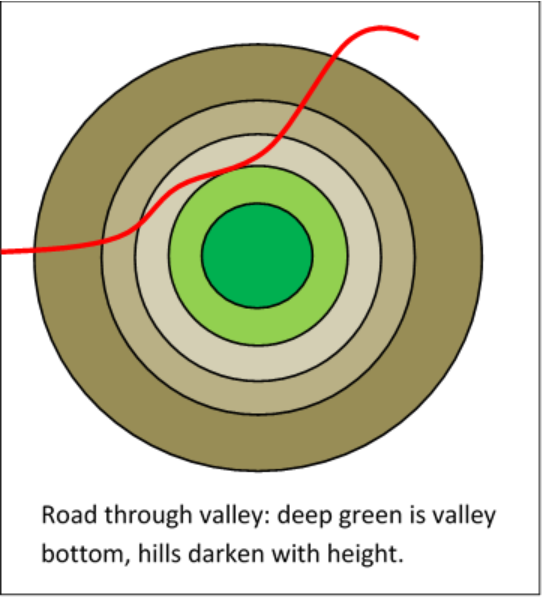
Let’s write the curve, the road, \(\begin{equation}
g(x, y)=0
\end{equation}\) (the wiggly red line in the figure below).

To find the closest approach point algebraically, we need to minimize \(\begin{equation}
f(x, y)=x^{2}+y^{2}
\end{equation}\) (square of distance to origin) subject to the constraint \(\begin{equation}
g(x, y)=0
\end{equation}\).

In the figure, we’ve drawn curves \begin{equation}
f(x, y)=x^{2}+y^{2}=a^{2}
\end{equation}

for a range of values of a (the circles centered at the origin). We need to find the point of intersection of \(\begin{equation}
g(x, y)=0
\end{equation}\) with the smallest circle it intersects—and it’s clear from the figure that it must touch that circle (if it crosses, it will necessarily get closer to the origin).

Therefore, at that point, the curves \(\begin{equation}
g(x, y)=0
\end{equation}\) and \(\begin{equation}
f(x, y)=a_{\min }^{2}
\end{equation}\) are parallel.

Therefore the normals to the curves are also parallel:

\begin{equation}
(\partial f / \partial x, \partial f / \partial y)=\lambda(\partial g / \partial x, \partial g / \partial y)
\end{equation}

(Note: yes, those are the directions of the normals— for an infinitesimal displacement along the curve \(\begin{equation}
f(x, y)=\text { constant }, 0=d f=(\partial f / \partial x) d x+(\partial f / \partial y) d y
\end{equation}\), so the vector \(\begin{equation}
(\partial f / \partial x, \partial f / \partial y)
\end{equation}\) is perpendicular to \(\begin{equation}
(d x, d y)
\end{equation}\). This is also analogous to the electric field \(\begin{equation}
\vec{E}=-\vec{\nabla} \varphi
\end{equation}\) being perpendicular to the equipotential \(\begin{equation}
\varphi(x, y)=\text { constant. })
\end{equation}\).

The constant \(\lambda\) introduced here is called a Lagrange multiplier. It’s just the ratio of the lengths of the two normal vectors (of course, “normal” here means the vectors are perpendicular to the curves, they are not normalized to unit length!) We can find \(\begin{equation}
\lambda
\end{equation}\) in terms of \(x\), \(y\) but at this point we don’t know their values.

The equations determining the closest approach to the origin can now be written:

\begin{equation}
\begin{array}{l}
\frac{\partial}{\partial x}(f-\lambda g)=0 \\
\frac{\partial}{\partial y}(f-\lambda g)=0 \\
\frac{\partial}{\partial \lambda}(f-\lambda g)=0
\end{array}
\end{equation}

(The third equation is just \(\begin{equation}
g\left(x_{\min }, y_{\min }\right)=0
\end{equation}\), meaning we’re on the road.)

We have transformed a constrained minimization problem in two dimensions to an unconstrained minimization problem in three dimensions! The first two equations can be solved to find \(\lambda\) and the ratio \(\begin{equation}
x / y
\end{equation}\) the third equation then gives \(x\), \(y\) separately.

Exercise for the reader: Work through this for \(\begin{equation}
g(x, y)=x^{2}-2 x y-y^{2}-1
\end{equation}\) (There are two solutions because the curve \(\begin{equation}
g=0
\end{equation}\) is a hyperbola with two branches.)

Lagrange multipliers are widely used in economics, and other useful subjects such as traffic optimization.