6.1: A Dynamical System’s Path in Configuration Space and in State Space

The story so far: For a mechanical system with n degrees of freedom, the spatial configuration at some instant of time is completely specified by a set of \(n\) variables we'll call the \(q_{i} \text { 's. }\). The n -dimensional \(q_{i}\) space is (naturally) called configuration space. It’s like a freeze frame, a snapshot of the system at a given instant. Subsequent time evolution from that state is uniquely determined if we're also given the initial velocities \(\dot{q}_{i}\).

The set of \(\begin{equation}
q_{i} \text { 's and } \dot{q}_{i} \text { 's }
\end{equation}\) together define the state of the system, meaning both its configuration and how fast it’s changing, therefore fully determining its future (and past) as well as its present. The 2n -dimensional space spanned by \(\begin{equation}
\left(q_{i}, \dot{q}_{i}\right)
\end{equation}\) is the state space.

The system’s time evolution is along a path in configuration space parameterized by the time t. That, of course, fixes the corresponding path in state space, since differentiating the functions \(\begin{equation}
q_{i}(t) \text { along that path determines the } \dot{q}_{i}(t)
\end{equation}\).

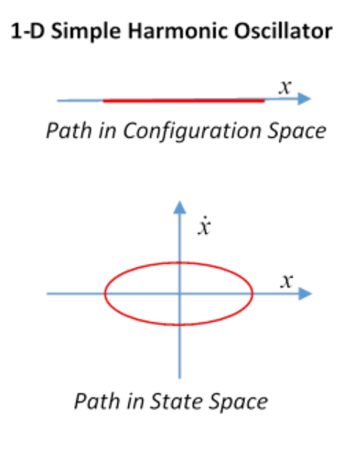
Trivial one-dimensional examples of these spaces are provided by the one-dimensional simple harmonic oscillator, where configuration space is just the x axis, say, the state space is the \(\begin{equation}
(x, \dot{x})
\end{equation}\) plane, the system’s time path in the state space is an ellipse.

For a stone falling vertically down, the configuration space is again a line, the path in the \(\begin{equation}
(x, \dot{x}) \text { state space is parabolic, } \dot{x} \propto \sqrt{x}
\end{equation}\).

Exercise: sketch the paths in state space for motions of a pendulum, meaning a mass at the end of a light rod, the other end fixed, but free to rotate in one vertical plane. Sketch the paths in \(\begin{equation}
(\theta, \dot{\theta})
\end{equation}\) coordinates.

In principle, the system’s path through configuration space can always be computed using Newton’s laws of motion, but in practice the math may be intractable. As we’ve shown above, the elegant alternative created by Lagrange and Hamilton is to integrate the Lagrangian

\begin{equation}
L\left(q_{i}, \dot{q}_{i}, t\right)=T\left(q_{i}, \dot{q}_{i}\right)-V\left(q_{i}, t\right)
\end{equation}

along different paths in configuration space from a given initial state to a given final state in a given time: as Hamilton proved, the actual path followed by the physical system between the two states in the given time is the one for which this integral, called the action, is minimized. This minimization, using the standard calculus of variations method, generates the Lagrange equations of motion in \(\begin{equation}
q_{i}, \dot{q}_{i}
\end{equation}\) and so determines the path.

Notice that specifying both the initial \(\begin{equation}
q_{i} \text { 's and the final } q_{i} \text { 's fixes } 2 n \text { variables. }
\end{equation}\). That’s all the degrees of freedom there are, so the motion is completely determined, just as it would be if we’d specified instead the initial \(\begin{equation}
q_{i} \text { 's and } \dot{q}_{i} \text { 's. }
\end{equation}\).