6.5: Math Note - the Legendre Transform

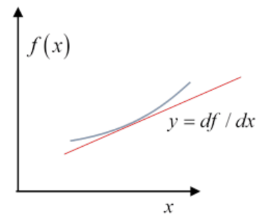
The change of variables described above is a standard mathematical routine known as the Legendre transform. Here’s the essence of it, for a function of one variable. Suppose we have a function \(f(x)\) that is convex, which is math talk for it always curves upwards, meaning \(d^{2} f(x) / d x^{2}\) is positive. Therefore its slope, we’ll call it

\[y=d f(x) / d x\]

is a monotonically increasing function of x. For some physics (and math) problems, this slope y, rather than the variable x, is the interesting parameter. To shift the focus to y, Legendre introduced a new function, \(g(y)\) defined by

\[g(y)=x y-f(x)\]

The function \(\begin{equation}
g(y)
\end{equation}\) is called the Legendre transform of the function \(\begin{equation}
f(x)
\end{equation}\).

To see how they relate, we take increments:

\[ \begin{align*} d g(y) &=y d x+x d y-d f(x) \\[4pt] &=y d x+x d y-y d x \\[4pt] &=x d y \end{align*}\]

(Looking at the diagram, an increment \(\begin{equation}
d x
\end{equation}\) gives a related increment \(\begin{equation}
d y
\end{equation}\) as the slope increases on moving up the curve.)

From this equation,

\begin{equation}
x=d g(y) / d y
\end{equation}

Comparing this with \(\begin{equation}
y=d f(x) / d x
\end{equation}\), it’s clear that a second application of the Legendre transformation would get you back to the original \(\begin{equation}
f(x)
\end{equation}\). So no information is lost in the Legendre transformation \(\begin{equation}
g(y)
\end{equation}\) in a sense contains \(\begin{equation}
f(x)
\end{equation}\), and vice versa.