23.2: The Road to Chaos

Equation of Motion

For the driven pendulum, the natural measure of the driving force is its ratio to the weight \(m g\), Taylor calls this the drive strength, so for driving force

\[F(t)=F_{0} \cos \omega t,\]

the drive strength \(\gamma\) is defined by

\[\gamma=F_{0} / m g.\]

The equation of motion (with resistive damping force \(-b v\) and hence resistive torque \(-b L^{2} \dot{\phi}\)) is:

\[m L^{2} \ddot{\phi}=-b L^{2} \dot{\phi}-m g L \sin \phi+L F(t)\]

Dividing by \(m L^{2}\) and writing the damping term \(b / m=2 \beta \) (to coincide with Taylor’s notation, his equation 12.12) we get (with \(\omega^2_0 = g/L\))

\[\ddot{\phi}+2 \beta \dot{\phi}+\omega_{0}^{2} \sin \phi=\gamma \omega_{0}^{2} \cos \omega t.\]

Behavior on Gradually Increasing the Driving Force: Period Doubling

The driving force \(\gamma=F_{0} / m g\) is the dimensionless ratio of drive strength to weight, so if this is small the pendulum will not be driven to large amplitudes, and indeed we find that after initial transients it settles to motion at the driving frequency, close to the linearized case. We would expect things to get more complicated when the oscillations have amplitude of order a radian, meaning a driving force comparable to the weight. And indeed they do.

Here we’ll show that our applet reproduces the sequence found by Taylor as the driving strength is increased.

In the equation of motion

\[\ddot{\phi}+2 \beta \dot{\phi}+\omega_{0}^{2} \sin \phi=\gamma \omega_{0}^{2} \cos \omega t,\]

We therefore choose his values \(\omega_{0}=1.5,2 \beta =0.75, \omega=1\) and gradually increase \(\gamma\) from \(0.9\) to \(1.0829\), where chaos begins.

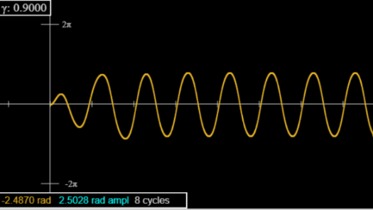
For \(\gamma=0.9,\) (see picture) the oscillation (after brief initial transients) looks like a sine wave, although it’s slightly flatter, and notice the amplitude (turquoise in box) is greater than \(\pi / 2\), the positive and negative swings are equal in magnitude to five figure accuracy after five or so oscillations.

You can see this for yourself by opening the applet! Click here. The applet plots the graph, and simultaneously shows the swinging pendulum (click bar at top right).

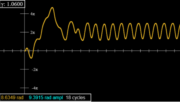
For \(\gamma=1.06\), there is a larger initial transient, vaguely resembling the three-cycle we’ll meet shortly. In fact, this can be suppressed by starting at \(\varphi=-\pi / 2\) (bottom slider on the right), but there are still transients: the peaks are not uniform to five-figure accuracy until about forty cycles.

For \(\gamma=1.0662\), there are very long transients: not evident on looking at the graph (on the applet), but revealed by monitoring the amplitude readout (turquoise figures in the box on the graph), the value at the most recent extremum. 

To get past these transients, set the applet speed to 50 (this does not affect accuracy, only prints a lot less dots). run 350 cycles then pause and go to speed = 2. You will find the peaks now alternate in height to the five-figure accuracy displayed, looks like period doubling—but it isn’t, run a few thousand cycles, if you have the patience, and you find all peaks have the same height. That was a long lived transient precursor of the period doubling transition.

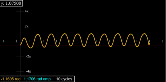
Going to 1.0664, you’ll see both peaks and dips now alternating in amplitude, for a well-defined period 2, which lasts until 1.0792. (Look at 1.075 after 70 or so cycles—and set the initial angle at -90.) 

Use the “ Red Line” slider just below the graph to check the heights of successive peaks or dips.

For \(\gamma =1.0793\), the period doubles again: successive peaks are now of order 0.4 radians apart, but successive “high” peaks are suddenly about 0.01 radians apart. (To see these better on the applet, magnify the vertical scale and move the red line.)

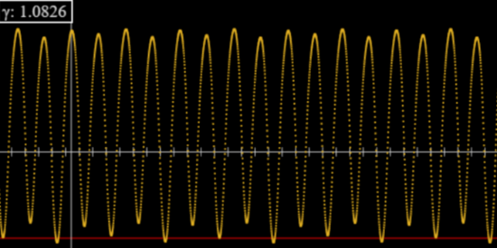
For \(\gamma=1.0821\) there is a further doubling to an 8 cycle, then at 1.0827 to a 16 cycle.

Look at the graph for 1.0826: in particular, the faint red horizontal line near the bottom. Every fourth dip goes below the line, but the next lowest dips alternate between touching the line and not quite reaching it. This is the 8 cycle.

It is known that the intervals between successive doublings decrease by a factor \(\delta = 4.6692\), found universally in period doubling cascades, and called the Feigenbaum number, after its discoverer. Our five-figure accuracy is too crude to follow this sequence further, but we can establish (or at least make very plausible!) that beyond the geometric series limit at \(\gamma_c=1.0829\) the periodicity disappears (temporarily, as we’ll see), the system is chaotic. (Of course, the values of \(\gamma\) depend on the chosen damping parameter, etc., only the ratio of doubling intervals is universal.)

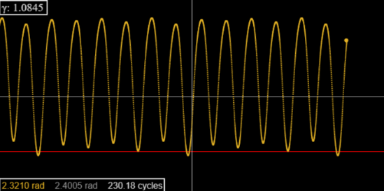
In fact, the full picture is complex: there are further intervals of periodicity, for example a 6 cycle at \(\gamma=1.0845\), pictured here.

Different Attractors

The periodic solutions described above are called “attractors”: configurations where the system settles down after initially wandering around. 

Clearly the attractors change with the driving strength, what is less obvious is that they may be different for different initial conditions. Taylor shows that for \(\gamma=1.077 \) taking \( \varphi(0)=0\) gives a 3-cycle after transients, but \(\varphi(0)=-\pi / 2\) gives a 2-cycle. (Easily checked with the applet!)

Looking at the initial wanderings, which can be quite different for very small changes in the driving strength (compare 1.0730 to 1.0729 and 1.0731, use speed 5, it doesn’t affect the accuracy). But you can see these initial wanderings include elements from both attractors.

Exercise: use the next applet to plot at the same time 1.0729 and 1.0730, all other parameters the same, speed 5.

Exercise: Use the applet to find at what angle the transition from one attractor to the other takes place. And, explore what happens over a range of driving strengths.

These are the simplest attractors: there are far more complex entities, called strange attractors, we’ll discuss later.

Exercises: Try different values of the damping constant and see how this affects the bifurcation sequence.

Sensitivity to Initial Conditions

Recall that for the linear damped driven oscillator, which can be solved exactly, we found that changing the initial conditions changed the path, of course, but the difference between paths decayed exponentially: the curves converged. 

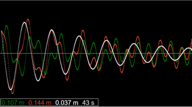
This illustration is from an earlier applet: the red and green curves correspond to different initial conditions, the white curve is the difference between the two, obviously exponentially decreasing, as can be verified analytically.

For the damped driven pendulum, the picture is more complicated. For \(\gamma<\gamma_{c}=1.0829\) curves corresponding to slightly different initial conditions will converge (except, for example, \(\gamma=1.077\) where, as mentioned above, varying the initial angle at a certain point switches form a final three-cycle to a two-cycle).

The Liapunov Exponent

For \(\gamma>\gamma_{c}\), curves even with very small initial differences (say, \(10^{-4}\) radians) separate exponentially, as \(e^{\lambda t}, \lambda\) is called the Liapunov exponent.

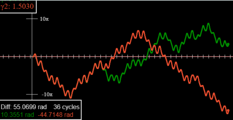
Bear in mind, though, that this is chaotic motion, the divergence is not as smooth as the convergence pictured above for the linear system. This graph is from our two-track applet.

Nevertheless, the (average) exponential nature can be discerned by plotting the logarithm of the difference against time:

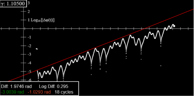
This is from our log difference applet. It is very close to Taylor’s fig 12.13. The red line slope gives the Lyapunov exponent.

(The red line has adjustable position and slope.)

Plotting Velocity against Time

As discussed in Taylor, further increase in the driving force beyond the chaotic threshold can lead to brief nonchaotic intervals, such as that containing the six cycle at 1.0845 illustrated above, but there are two long stretches of nonchaotic behavior in Taylor’s parameter range, from 1.1098 to 1.1482 and from 1.3 to 1.48.

In the stronger driving force range, the pendulum is driven completely around in each cycle, so plotting the position against time gives a “rounded staircase” kind of graph. Check this with the applet.

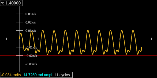
The solution is to plot velocity against time, and thereby discover that there is a repetition of the period doubling route to chaos at the upper end of this interval. Click to plot \(d\phi /dt\) instead of \(\phi\).

 

State-Space Trajectories

It can be illuminating to watch the motion develop in time in the two-dimensional state space (\(\phi, \dot{\phi}\)). (Equally called phase space.) See the State Space applet!

Now for a particle in a time-independent potential, specifying position and velocity at a given instant determines the future path—but that is not the case here, the acceleration is determined by the phase of the driving force, which is time varying, so the system really needs three parameters to specify its subsequent motion. 

That means the phase space is really three-dimensional, the third direction being the driving phase, or, equivalently, time, but periodic with the period of the driving force. In this three-dimensional space, paths cannot cross, at any point the future path is uniquely defined. Our two-dimensional plots are projections of these three-dimensional paths on to the (\(\phi, \dot{\phi}\)) plane.

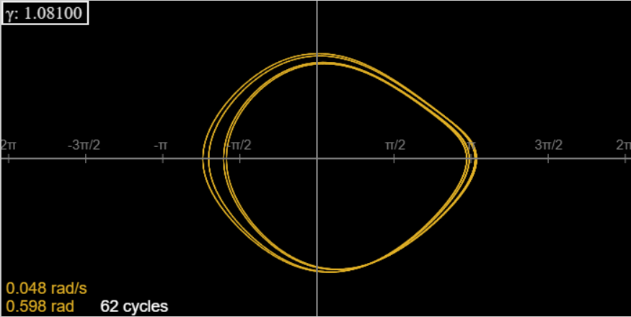
Here’s the 4-cycle at \(\gamma = 1.081\), minus the first 20 cycles, to eliminate transients.

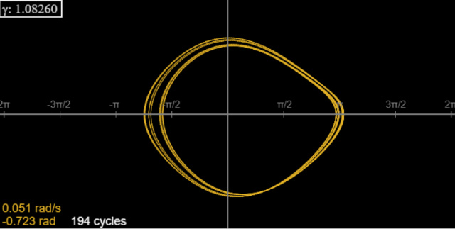
For \(\gamma = 1.0826\), there is an 8-cycle. Run the applet for 40 cycles or so to get rid of transients, then look at the far-left end of the curve generated by running, say, to 200 cycles. It doesn’t look like there are 8 lines, but the outermost line and the two innermost lines are doubles (notice the thickness). You can check this with the applet, by pausing at the axis and noticing the position readout: there are 8 different values that repeat. (You don’t have to stop right on the axis—you can stop close to it, then use the step buttons to get there.)

For \(\gamma = 1.0830\), the path is chaotic—but doesn’t look too different on this scale! Check it out with the applet. The chaos becomes more evident on further increasing \(\gamma\). For \(\gamma =1.087\) the pattern is “fattened” as repeated cycles differ slightly.

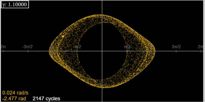
For further increase in \(\gamma\), the orbital motion covers more territory: at \(\gamma = 1.1\), here are the first three hundred or so cycles.

Plotting many orbits at high speed we find:

However, here the story gets complicated: it turns out that this chaotic series of orbits is in fact a transient, and after about 300 cycles the system skips to a 3-cycle, where it stays. In fact, we have reached a range of \(\gamma\) (approximately 1.1098 to 1.1482) where after initial transients (which can be quite long) the motion is not chaotic, but a 3-cycle.

Obviously, there is a lot to explore for this system! To get a better grasp of these complexities, we try a different approach, developed by Poincaré.

Poincaré Sections

Looking at the above pictures, as we go from a single orbit to successive period doublings and then chaos, the general shape of the orbit doesn’t change dramatically (until that final three-cycle). The interesting things are the doubling sequence, chaos, and attractors—perhaps we’re plotting too much information.

To focus on what’s essential, Poincaré plotted a single point from each cycle, this is now called a Poincaré section. To construct this, we begin with the \(t = 0\) position, label it \(P_0=(\varphi_0,\dot{\varphi}_0)\). Then add the point \(P_1=(\varphi_1,\dot{\varphi}_1)\) precisely one cycle later, and so on—points one cycle apart, \(P_2=(\varphi_2,\dot{\varphi}_2)\), etc. Now, knowing the position \(P=(\varphi,\dot{\varphi})\) in state space is not enough information to plot the future orbit—we also need to know the phase of the driving force. But by plotting points one cycle in time apart, they will all see the same phase starting force, so the transformation that takes us from \(P_0\) to \(P_1\) just repeats in going from \(P_1\) to \(P_2\), etc.

To see these single points in the State Space applet, click “Show Red Dot”: on running, the applet will show one dot per cycle red.

Thinking momentarily of the full three-dimensional phase space, the Poincaré section is a cross-section at the initial phase of the driving cycle. We’ve added to the applet a red dot phase option, to find the Poincaré section at a different phase. Doing this a few times, and looking at the movement of the red dots, gives a fuller picture of the motion.

So the Poincaré section, on increasing \(\gamma\) through the doubling sequence (and always omitting initial transients) goes from a single point to two points, to four, etc.

To see all this a bit more clearly, the next applet, called Poincaré Section, shows only one dot per cycle, but has a phase option so you can look at any stage in the cycle.

Exercise: check this all out with the Poincaré applet! To see it well, click Toggle Origin/Scale, use the sliders to center the pattern, more or less, then scale it up. Run for a few hundred cycles, then click Hide Trace followed by Show Trace to get rid of transients.

Start with \(\gamma = 1.0826\). The Poincaré section is eight points on a curve, at 1.0827 you can discern 16. By 1.0829, we have chaos, and the section has finite stretches of the curve, not just points. It looks very similar at 1.0831, but—surprise—at 1.0830 it’s a set of points (32?) some doubled. This tells us we’re in a minefield. There’s nothing smooth about chaos.

Apart from interruptions, as \(\gamma\) increases, the Poincaré section fills a curve, which then evolves towards the strange attractor shown by Taylor and others. Going from 1.090 in steps to 1.095, the curve evolves a second, closely parallel, branch. At 1.09650 the two branches are equal in length, then at 1.097 the lower branch suddenly extends a long curve, looks much the same at 1.100, then by 1.15 we recognize the emergence of the strange attractor.

But in fact this is a simplified narrative: there are interruptions. For example, at \(\gamma = 1.0960\) there’s a 5-cycle, no chaos (it disappears on changing by 0.0001). And at 1.12 we’re in the 3-cycle interval mentioned earlier.

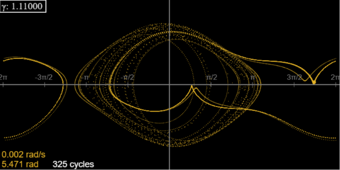
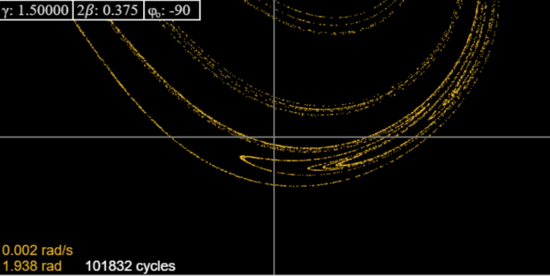
Anyway, the strange attractor keeps reappearing, and at 1.5 it looks like this:

This looks rather thin compared to Taylor’s picture for the same \(\gamma\): the reason is we have kept the strong damping.

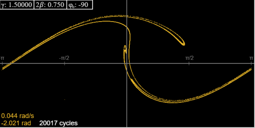
Changing to \(2\beta =0.375\), we recover Taylor’s picture. Like him, we show here (from the applet) the attractor and successive magnifications of one part, to give some hint of the fractal structure:

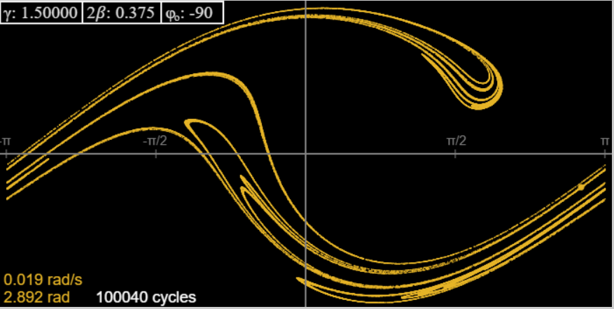
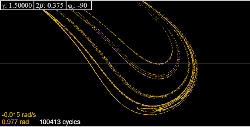
We have to admit that at the highest magnification Taylor’s picture is certainly superior to that generated by the applet, but does not contradict it—actually, it reassures us that the applet is reliable up to the level of definition that is self-evident on looking at it.

Exercise: Use the last two applets to explore other regions of parameter space. What happens on varying the damping? Going from \(2\beta =0.375\) to \(2\beta =0.75\) the attractor has the same general form but is much narrower. Then go in 0.001 steps to 0.76. For some values you see the attractor, but for others a cycle, different lengths. There is a two-cycle from 0.76 to 0.766, then a four cycle, then at 0.78 back to a two-cycle, at 0.814 a one-cycle. If you up the driving strength, and the damping, you can find extremely narrow attractors.

Exercise: Baker and Gollub, Chaotic Dynamics, page 52, give a sequence of Poincaré sections at \(0.2\pi\) intervals for \(\gamma=1.5\) and \(2\beta =0.75\). You can check them (and intermediate ones) with the applet, and try to imagine putting them in a stack to visualize the full three-dimensional attractor!