
5.7: Constrained Variational Systems


- Last updated
- Mar 14, 2021
- Save as PDF

( \newcommand{\kernel}{\mathrm{null}\,}\)
Imposing a constraint on a variational system implies:
- The N constrained coordinates yi(x) are correlated which violates the assumption made in chapter 5.5 that the N variables are independent.
- Constrained motion implies that constraint forces must be acting to account for the correlation of the variables. These constraint forces must be taken into account in the equations of motion.
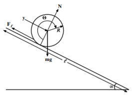
For example, for a disk rolling down an inclined plane without slipping, there are three coordinates x [perpendicular to the wedge], y, [Along the surface of the wedge], and the rotation angle θ shown in Figure 5.7.1. The constraint forces, Ff N, lead to the correlation of the variables such that x=R, while y=Rθ. Basically there is only one independent variable, which can be either y or θ. The use of only one independent variable essentially buries the constraint forces under the rug, which is fine if you only need to know the equation of motion. If you need to determine the forces of constraint then it is necessary to include all coordinates explicitly in the equations of motion as discussed below.
Holonomic constraints
Most systems involve restrictions or constraints that couple the coordinates. For example, the yi(x) may be confined to a surface in coordinate space. The constraints mean that the coordinates yi(x) are not independent, but are related by equations of constraint. A constraint is called holonomic if the equations of constraint can be expressed in the form of an algebraic equation that directly and unambiguously specifies the shape of the surface of constraint. A non-holonomic constraint does not provide an algebraic relation between the correlated coordinates. In addition to the holonomy of the constraints, the equations of constraint also can be grouped into the following three classifications depending on whether they are algebraic, differential, or integral. These three classifications for the constraints exhibit different holonomy relating the coupled coordinates. Fortunately the solution of constrained systems is greatly simplified if the equations of constraint are holonomic.
Geometric (algebraic) equations of constraint
Geometric constraints can be expressed in the form of algebraic relations that directly specify the shape of the surface of constraint in coordinate space q1,q2,…,qj,..qn.
gk(q1,q2,..qj,..qn;t)=0
where j=1,2,3,…n. There can be m such equations of constraint where 0≤k≤m. An example of such a geometric constraint is when the motion is confined to the surface of a sphere of radius R in coordinate space which can be written in the form g=x2+y2+z2−R2=0. Such algebraic constraint equations are called Holonomic which allows use of generalized coordinates as well as Lagrange multipliers to handle both the constraint forces and the correlation of the coordinates.
Kinematic (differential) equations of constraint
The m constraint equations also can be expressed in terms of the infinitessimal displacements of the form
n∑j=1∂gk∂qjdqj+∂gk∂tdt=0
where k=1,2,3,…m, j=1,2,3,…n. If Equation ??? represents the total differential of a function then it can be integrated to give a holonomic relation of the form of Equation ???. However, if Equation ??? is not the total differential, then it is non-holonomic and can be integrated only after having solved the full problem.
An example of differential constraint equations is for a wheel rolling on a plane without slipping which is non-holonomic and more complicated than might be expected. The wheel moving on a plane has five degrees of freedom since the height z is fixed. That is, the motion of the center of mass requires two coordinates (x,y) plus there are three angles (ϕ,θ,ψ) where ϕ is the rotation angle for the wheel, θ is the pivot angle of the axis, and ψ is the tilt angle of the wheel. If the wheel slides then all five degrees of freedom are active. If the axis of rotation of the wheel is horizontal, that is, the tilt angle ψ=0 is constant, then this kinematic system leads to three differential constraint equations The wheel can roll with angular velocity ˙ϕ, as well as pivot which corresponds to a change in θ. Combining these leads to two differential equations of constraint
dx−asinθdϕ=0dy+acosθdϕ=0
These constraints are insufficient to provide finite relations between all the coordinates. That is, the constraints cannot be reduced by integration to the form of Equation ??? because there is no functional relation between ϕ and the other three variables, x,y,θ. Many rolling trajectories are possible between any two points of contact on the plane that are related to different pivot angles. That is, the point of contact of the disk could pivot plus roll in a circle returning to the same point where x,y,θ are unchanged whereas the value of ϕ depends on the circumference of the circle. As a consequence the rolling constraint is non-holonomic except for the case where the disk rolls in a straight line and remains vertical.
Isoperimetric (integral) equations of constraint
Equations of constraint also can be expressed in terms of direct integrals. This situation is encountered for isoperimetric problems, such as finding the maximum volume bounded by a surface of fixed area, or the shape of a hanging rope of fixed length. Integral constraints occur in economics when minimizing some cost algorithm subject to a fixed total cost constraint.
A simple example of an isoperimetric problem involves finding the curve y=y(x) such that the functional has an extremum where the curve y(x) satisfies boundary conditions such that y(x1)=a and y(x2)=b, that is
F(y)=∫x2x1f(y,y′;x)dx
is an extremum such that the perimeter also is constrained to satisfy
G(y)=∫x2x1g(y,y′;x)dx=l
where l is a fixed length. This integral constraint is geometric and holonomic. Another example is finding the minimum surface area of a closed surface subject to the enclosed volume being the constraint.
Properties of the constraint equations
Holonomic constraints
Geometric constraints can be expressed in the form of an algebraic equation that directly specifies the shape of the surface of constraint
g(y1,y2,y3,…;x)=0
Such a system is called holonomic since there is a direct relation between the coupled variables. An example of such a holonomic geometric constraint is if the motion is confined to the surface of a sphere of radius R which can be written in the form g=x2+y2+z2−R2=0
Non-holonomic constraints
There are many classifications of non-holonomic constraints that exist if Equation ??? is not satisfied. The algebraic approach is difficult to handle when the constraint is an inequality, such as the requirement that the location is restricted to lie inside a spherical shell of radius R which can be expressed as
g=x2+y2+z2−R2≤0
This non-holonomic constrained system has a one-sided constraint. Systems usually are non-holonomic if the constraint is kinematic as discussed above.
Partial Holonomic constraints
Partial-holonomic constraints are holonomic for a restricted range of the constraint surface in coordinate space, and this range can be case specific. This can occur if the constraint force is one-sided and perpendicular to the path. An example is the pendulum with the mass attached to the fulcrum by a flexible string that provides tension but not compression. Then the pendulum length is constant only if the tension in the string is positive. Thus the pendulum will be holonomic if the gravitational plus centrifugal forces are such that the tension in the string is positive, but the system becomes non-hononomic if the tension is negative as can happen when the pendulum rotates to an upright angle where the centrifugal force outwards is insufficient to compensate for the vertical downward component of the gravitational force. There are many other examples where the motion of an object is holonomic when the object is pressed against the constraint surface, such as the surface of the Earth, but is unconstrained if the object leaves the surface.
Time dependence
A constraint is called scleronomic if the constraint is not explicitly time dependent. This ignores the time dependence contained within the solution of the equations of motion. Fortunately a major fraction of systems are scleronomic. The constraint is called rheonomic if the constraint is explicitly time dependent. An example of a rheonomic system is where the size or shape of the surface of constraint is explicitly time dependent such as a deflating pneumatic tire.
Energy Conservation
The solution depends on whether the constraint is conservative or dissipative, that is, if friction or drag are acting. The system will be conservative if there are no drag forces, and the constraint forces are perpendicular to the trajectory of the path such as the motion of a charged particle in a magnetic field. Forces of constraint can result from sliding of two solid surfaces, rolling of solid objects, fluid flow in a liquid or gas, or result from electromagnetic forces. Energy dissipation can result from friction, drag in a fluid or gas, or finite resistance of electric conductors leading to dissipation of induced electric currents in a conductor, e.g. eddy currents.
A rolling constraint is unusual in that friction between the rolling bodies is necessary to maintain rolling. A disk on a frictionless inclined plane will conserve it’s angular momentum since there is no torque acting if the rolling contact is frictionless, that is, the disk will just slide. If the friction is sufficient to stop sliding, then the bodies will roll and not slide. A perfect rolling body does not dissipate energy since no work is done at the instantaneous point of contact where both bodies are in zero relative motion and the force is perpendicular to the motion. In real life, a rolling wheel can involve a very small energy dissipation due to deformation at the point of contact coupled with non-elastic properties of the material used to make the wheel and the plane surface. For example, a pneumatic tire can heat up and expand due to flexing of the tire.
Treatment of constraint forces in variational calculus
There are three major approaches to handle constraint forces in variational calculus. All three of them exploit the tremendous freedom and flexibility available when using generalized coordinates. The (1) generalized coordinate approach, described in chapter 5.8, exploits the correlation of the n coordinates due to the m constraint forces to reduce the dimension of the equations of motion to s=n−m degrees of freedom. This approach embeds the m constraint forces, into the choice of generalized coordinates and does not determine the constraint forces, (2) Lagrange multiplier approach, described in chapter 5.9, exploits generalized coordinates but includes the m constraint forces into the Euler equations to determine both the constraint forces in addition to the n equations of motion. (3) Generalized forces approach, described in chapter 6.7.3, introduces constraint and other forces explicitly.