5.9: Lagrange multipliers for Holonomic Constraints

Algebraic equations of constraint

The Lagrange multiplier technique provides a powerful, and elegant, way to handle holonomic constraints using Euler’s equations¹. The general method of Lagrange multipliers for \(n\) variables, with \(m\) constraints, is best introduced using Bernoulli’s ingenious exploitation of virtual infinitessimal displacements, which Lagrange signified by the symbol \(\delta\). The term "virtual" refers to an intentional variation of the generalized coordinates \(\delta q_{i}\) in order to elucidate the local sensitivity of a function \(F(q_{i},x)\) to variation of the variable. Contrary to the usual infinitessimal interval in differential calculus, where an actual displacement \(dq_{i}\) occurs during a time \(dt\), a virtual displacement is imagined to be an instantaneous, infinitessimal, displacement of a coordinate, not an actual displacement, in order to elucidate the local dependence of \(F\) on the coordinate. The local dependence of any functional \(F,\) to virtual displacements of all \(n\) coordinates, is given by taking the partial differentials of \(F\).

\[\delta F=\sum_{i}^{n}\frac{\partial F}{\partial q_{i}}\delta q_{i} \label{5.35}\]

The function \(F\) is stationary, that is an extremum, if Equation \ref{5.35} equals zero. The extremum of the functional \(F\), given by equation (\(5.5.1\)), can be expressed in a compact form using the virtual displacement formalism as \[\delta F=\delta \int_{x_{1}}^{x_{2}}\sum_{i}^{n}f\left[ q_{i}(x),q_{i}^{\prime }(x);x\right] dx=\sum_{i}^{n}\frac{\partial F}{\partial q_{i}}\delta q_{i}=0\label{5.36}\]

The auxiliary conditions, due to the \(m\) holonomic algebraic constraints for the \(n\) variables \(q_{i}\), can be expressed by the \(m\) equations

\[g_{k}(\mathbf{q})=0\label{5.37}\]

where \(1\leq k\leq m\) and \(1\leq i\leq n\) with \(m<n\). The variational problem for the \(m\) holonomic constraint equations also can be written in terms of \(m\) differential equations where \(1\leq k\leq m\) \[\delta g_{k}=\sum_{i=1}^{n}\frac{\partial g_{k}}{\partial q_{i}}\delta q_{i}=0\label{5.38}\]

Since equations \ref{5.36} and \ref{5.38} both equal zero, the \(m\) equations \ref{5.38} can be multiplied by arbitrary undetermined factors \(\lambda _{k},\) and added to equations \ref{5.36} to give.

\[\delta F(q_{i},x)+\lambda _{1}\delta g_{1}+\lambda _{2}\delta g_{2}\cdot \cdot \lambda _{k}\delta g_{k}\cdot \cdot \lambda _{m}\delta g_{m}=0\label{5.39}\]

Note that this is not trivial in that although the sum of the constraint equations for each \(y_{i\text{ }}\)is zero; the individual terms of the sum are not zero.

Insert equations \ref{5.36} plus \ref{5.38} into \ref{5.39}, and collect all \(n\) terms, gives \[\sum_{i}^{n}\left( \frac{\partial F}{\partial q_{i}}+\sum_{k=1}^{m}\lambda _{k}\frac{\partial g_{k}}{\partial q_{i}}\right) \delta q_{i}=0\label{5.40}\]

Note that all the \(\delta q_{i}\) are free independent variations and thus the terms in the brackets, which are the coefficients of each \(\delta q_{i}\), individually must equal zero. For each of the \(n\) values of \(i\), the corresponding bracket implies

\[\frac{\partial F}{\partial q_{i}}+\sum_{k=1}^{m}\lambda _{k}\frac{\partial g_{k}}{\partial q_{i}}=0\label{5.41}\]

This is equivalent to what would be obtained from the variational principle

\[\delta F+\sum_{k=1}^{m}\lambda _{k}\delta g_{k}=0\label{5.42}\]

Equation \ref{5.42} is equivalent to a variational problem for finding the stationary value of \(F^{\prime }\)

\[\delta \left( F^{\prime }\right) =\delta \left( F+\sum_{k}^{m}\lambda _{k}g_{k}\right) =0\label{5.43}\]

where \(F^{\prime }\) is defined to be

\[F^{\prime }\equiv \left( F+\sum_{k=1}^{m}\lambda _{k}g_{k}\right)\label{5.44}\]

The solution to Equation \ref{5.43} can be found using Euler’s differential equation (\(5.5.4\)) of variational calculus. At the extremum \(\delta \left( F^{\prime }\right) =0\) corresponds to following contours of constant \(F^{\prime }\) which are in the surface that is perpendicular to the gradients of the terms in \(F^{\prime }\). The Lagrange multiplier constants are required because, although these gradients are parallel at the extremum, the magnitudes of the gradients are not equal.

The beauty of the Lagrange multipliers approach is that the auxiliary conditions do not have to be handled explicitly, since they are handled automatically as \(m\) additional free variables during solution of Euler’s equations for a variational problem with \(n+m\) unknowns fit to \(n+m\) equations. That is, the \(n\) variables \(q_{i}\) are determined by the variational procedure using the \(n\) variational equations

\[\frac{d}{dx}(\frac{\partial F^{\prime }}{\partial q_{i}^{\prime }})-(\frac{\partial F^{\prime }}{\partial q_{i}})=\frac{d}{dx}(\frac{\partial F}{\partial q_{i}^{\prime }})-(\frac{\partial F}{\partial q_{i}})-\sum_{k}^{m}\lambda _{k}\frac{\partial g_{k}}{\partial q_{i}}=0 \label{5.45}\]

simultaneously with the \(m\) variables \(\lambda _{k}\) which are determined by the \(m\) variational equations

\[\frac{d}{dx}(\frac{\partial F^{\prime }}{\partial \lambda _{k}^{\prime }})-(\frac{\partial F^{\prime }}{\partial \lambda _{k}})=0\label{5.46}\]

Equation \ref{5.45} usually is expressed as

\[(\frac{\partial F}{\partial q_{i}})-\frac{d}{dx}(\frac{\partial F}{\partial q_{i}^{\prime }})+\sum_{k}^{m}\lambda _{k}\frac{\partial g_{k}}{\partial q_{i}}=0 \label{5.47}\]

The elegance of Lagrange multipliers is that a single variational approach allows simultaneous determination of all \(n+m\) unknowns. Chapter \(6.2\) shows that the forces of constraint are given directly by the \(\lambda _{k}\frac{\partial g_{k}}{\partial q_{i}}\) terms.

Example \(\PageIndex{1}\): Two dependent variables coupled by one holonomic constraint

The powerful, and generally applicable, Lagrange multiplier technique is illustrated by considering the case of only two dependent variables, \(y(x),\) and \(z\left( x\right) ,\) with the function \(f(y(x),y^{\prime }(x),z(x),z(x)^{\prime };x)\) and with one holonomic equation of constraint coupling these two dependent variables. The extremum is given by requiring

\[\frac{\partial F}{\partial \epsilon }=\int_{x_{1}}^{x_{2}}\left[ \left( \frac{\partial f}{\partial y}-\frac{d}{dx}\frac{\partial f}{\partial y^{\prime }}\right) \frac{\partial y}{\partial \epsilon }+\left( \frac{\partial f}{\partial z}-\frac{d}{dx}\frac{\partial f}{\partial z^{\prime }}\right) \frac{\partial z}{\partial \epsilon }\right] dx=0 \tag{$A$} \label{A}\]

with the constraint expressed by the auxiliary condition

\[g\left( y,z;x\right) =0 \tag{$B$} \label{B}\]

Note that the variations \(\frac{\partial y}{\partial \epsilon }\) and \(\frac{\partial z}{\partial \epsilon }\) are no longer independent because of the constraint equation, thus the the two terms in the brackets of Equation \ref{A} are not separately equal to zero at the extremum. However, differentiating the constraint Equation \ref{B} gives

\[\frac{dg}{d\epsilon }=\left( \frac{\partial g}{\partial y}\frac{\partial y}{\partial \epsilon }+\frac{\partial g}{\partial z}\frac{\partial z}{\partial \epsilon }\right) =0 \tag{$C$} \label{C}\]

No \(\frac{\partial g}{\partial x}\) term applies because, for the independent variable, \(\frac{\partial x}{\partial \epsilon }\) \(=0.\) Introduce the neighboring paths by adding the auxiliary functions

\[\begin{align} y(\epsilon ,x) &=&y(x)+\epsilon \eta _{1}(x) \tag{$D$} \label{D} \\ z(\epsilon ,x) &=&z(x)+\epsilon \eta _{2}(x) \tag{$E$} \label{E}\end{align}\]

Insert the differentials of equations \ref{D} and \ref{E} , into \ref{C} gives

\[\frac{dg}{d\epsilon }=\left( \frac{\partial g}{\partial y}\eta _{1}(x)+\frac{\partial g}{\partial z}\eta _{2}(x)\right) =0 \tag{$F$} \label{F}\]

implying that

\[\eta _{2}(x)=-\frac{\frac{\partial g}{\partial y}}{\frac{\partial g}{\partial z}}\eta _{1}(x) \nonumber\]

Equation \ref{A} can be rewritten as

\[\begin{align} \int_{x_{1}}^{x_{2}}\left[ \left( \frac{\partial f}{\partial y}-\frac{d}{dx}\frac{\partial f}{\partial y^{\prime }}\right) \eta _{1}(x)+\left( \frac{\partial f}{\partial z}-\frac{d}{dx}\frac{\partial f}{\partial z^{\prime }}\right) \eta _{2}(x)\right] dx &=&0 \notag \\ \int_{x_{1}}^{x_{2}}\left[ \left( \frac{\partial f}{\partial y}-\frac{d}{dx}\frac{\partial f}{\partial y^{\prime }}\right) -\left( \frac{\partial f}{\partial z}-\frac{d}{dx}\frac{\partial f}{\partial z^{\prime }}\right) \frac{\frac{\partial g}{\partial y}}{\frac{\partial g}{\partial z}}\right] \eta _{1}(x)dx &=&0 \tag{$G$} \label{G}\end{align}\]

Equation \ref{G} now contains only a single arbitrary function \(\eta _{1}(x)\) that is not restricted by the constraint. Thus the bracket in the integrand of Equation \ref{G} must equal zero for the extremum. That is

\[\left( \frac{\partial f}{\partial y}-\frac{d}{dx}\frac{\partial f}{\partial y^{\prime }}\right) \left( \frac{\partial g}{\partial y}\right) ^{-1}=\left( \frac{\partial f}{\partial z}-\frac{d}{dx}\frac{\partial f}{\partial z^{\prime }}\right) \left( \frac{\partial g}{\partial z}\right) ^{-1}\equiv -\lambda (x) \notag\]

Now the left-hand side of this equation is only a function of \(f\) and \(g\) with respect to \(y\) and \(y^{\prime }\) while the right-hand side is a function of \(f\) and \(g\) with respect to \(z\) and \(z^{\prime }.\) Because both sides are functions of \(x\) then each side can be set equal to a function \(-\lambda (x).\) Thus the above equations can be written as

\[\frac{d}{dx}\frac{\partial f}{\partial y^{\prime }}-\frac{\partial f}{\partial y}=\lambda \left( x\right) \frac{\partial g}{\partial y}\hspace{1in}\frac{d}{dx}\frac{\partial f}{\partial z^{\prime }}-\frac{\partial f}{\partial z}=\lambda \left( x\right) \frac{\partial g}{\partial z} \tag{$H$} \label{H}\]

The complete solution of the three unknown functions. \(y(x),z(x),\) and \(\lambda (x).\) is obtained by solving the two equations, \ref{H}, plus the equation of constraint \ref{F}. The Lagrange multiplier \(\lambda (x)\) is related to the force of constraint. This example of two variables coupled by one holonomic constraint conforms with the general relation for many variables and constraints given by Equation \ref{5.47}.

Integral equations of constraint

The constraint equation also can be given in an integral form which is used frequently for isoperimetric problems . Consider a one dependent-variable isoperimetric problem, for finding the curve \(q=q(x)\) such that the functional has an extremum, and the curve \(q(x)\) satisfies boundary conditions such that \(q(x_{1})=a\) and \(q(x_{2})=b\). That is

\[F(y)=\int_{x_{1}}^{x_{2}}f(q,q^{\prime };x)dx\]

is an extremum such that the fixed length \(l\) of the perimeter satisfies the integral constraint \[G(y)=\int_{x_{1}}^{x_{2}}g(q,q^{\prime };x)dx=l\]

Analogous to \ref{5.44} these two functionals can be combined requiring that

\[\delta K(q,x,\lambda )\equiv \delta \left[ F(q)+\lambda G(q)\right] =\delta \int_{x_{1}}^{x_{2}}[f+\lambda g]dx=0\]

That is, it is an extremum for both \(q(x)\) and the Lagrange multiplier \(\lambda\). This effectively involves finding the extremum path for the function \(K(q,x,\lambda )=F(q,x)+\lambda G(q,x)\) where both \(q(x)\) and \(\lambda\) are the minimized variables. Therefore the curve \(q(x)\) must satisfy the differential equation

\[\frac{d}{dx}\frac{\partial f}{\partial q_{i}^{\prime }}-\frac{\partial f}{\partial q_{i}}+\lambda \left[ \frac{d}{dx}\frac{\partial g}{\partial q_{i}^{\prime }}-\frac{\partial g}{\partial q_{i}}\right] =0 \label{5.51}\]

subject to the boundary conditions \(q(x_{1})=a,\) \(q(x_{2})=b,\) and \(G(q)=l\).

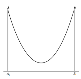
Example \(\PageIndex{2}\): Catenary

One isoperimetric problem is the catenary which is the shape a uniform rope or chain of fixed length \(l\) that minimizes the gravitational potential energy. Let the rope have a uniform mass per unit length of \(\sigma\) kg/m\(.\)

Figure \(\PageIndex{1}\): The catenary

The gravitational potential energy is

\[U=\sigma g\int_{1}^{2}yds=\sigma g\int_{1}^{2}y\sqrt{dx^{2}+dy^{2}}=\sigma g\int_{1}^{2}y\sqrt{1+y^{\prime 2}}dx \notag\]

The constraint is that the length be a constant \(l\)

\[l=\int_{1}^{2}ds=\int_{1}^{2}\sqrt{1+y^{\prime 2}}dx \notag\]

Thus the function is \(f(y,y^{\prime };x)=y\sqrt{1+y^{\prime 2}}\) while the integral constraint sets \(g=\sqrt{1+y^{\prime 2}}\)

These need to be inserted into the Euler Equation \ref{5.51} by defining

\[F=f+\lambda g=(y+\lambda )\sqrt{1+y^{\prime 2}}\nonumber\]

Note that this case is one where \(\frac{\partial F}{\partial x}=0\) and \(\lambda\) is a constant; also defining \(z=y+\lambda\) then \(z^{\prime }=y^{\prime }.\) Therefore the Euler’s equations can be written in the integral form

\[F-z^{\prime }\frac{\partial F}{\partial z^{\prime }}=c=\text{constant}\nonumber\]

Inserting the relation \(F=z\sqrt{1+z^{\prime 2}}\) gives

\[z\sqrt{1+z^{\prime 2}}-z^{\prime }\frac{zz^{\prime }}{\sqrt{1+z^{\prime 2}}}=c\nonumber\]

where \(c\) is an arbitrary constant. This simplifies to

\[z^{\prime 2}=\left( \frac{z}{c}\right) ^{2}-1\nonumber\]

The integral of this is

\[z=c\cosh \left( \frac{x+b}{c}\right)\nonumber\]

where \(b\) and \(c\) are arbitrary constants fixed by the locations of the two fixed ends of the rope.

Example \(\PageIndex{3}\): The Queen Dido problem

A famous constrained isoperimetric legend is that of Dido, first Queen of Carthage. Legend says that, when Dido landed in North Africa, she persuaded the local chief to sell her as much land as an oxhide could contain. She cut an oxhide into narrow strips and joined them to make a continuous thread more than four kilometers in length which was sufficient to enclose the land adjoining the coast on which Carthage was built. Her problem was to enclose the maximum area for a given perimeter. Let us assume that the coast line is straight and the ends of the thread are at \(\pm a\) on the coast line. The enclosed area is given by

\[A=\int_{-a}^{+a}ydx\nonumber\]

The constraint equation is that the total perimeter equals \(l\).

\[\int_{-a}^{a}\sqrt{1+y^{\prime 2}}dx=l\nonumber\]

Thus we have that the functional \(f(y,y^{\prime },x)=y\) and \(g(y,y^{\prime },x)=\sqrt{1+y^{\prime 2}}\). Then \(\frac{\partial f}{\partial y}=1,\frac{\partial f}{\partial y^{\prime }}=0,\frac{\partial g}{\partial y}=0\) and \(\frac{\partial g}{\partial y^{\prime }}=\frac{y^{\prime }}{\sqrt{1+y^{\prime 2}}}.\) Insert these into the Euler-Lagrange Equation \ref{5.51} gives

\[1-\lambda \frac{d}{dx}\left[ \frac{y^{\prime }}{\sqrt{1+y^{\prime 2}}}\right] =0\nonumber\]

That is

\[\frac{d}{dx}\left[ \frac{y^{\prime }}{\sqrt{1+y^{\prime 2}}}\right] =\frac{1}{\lambda }\nonumber\]

Integrate with respect to \(x\) gives

\[\frac{\lambda y^{\prime }}{\sqrt{1+y^{\prime 2}}}=x-b\nonumber\]

where \(b\) is a constant of integration. This can be rearranged to give

\[y^{\prime }=\frac{\pm \left( x-b\right) }{\sqrt{\lambda ^{2}-\left( x-b\right) ^{2}}}\nonumber\]

The integral of this is

\[y=\mp \sqrt{\lambda ^{2}-\left( x-b\right) ^{2}}+c\nonumber\]

Rearranging this gives

\[\left( x-b\right) ^{2}+\left( y-c\right) ^{2}=\lambda ^{2}\nonumber\]

This is the equation of a circle centered at \((b,c)\). Setting the bounds to be \(\left( -a,0\right)\) to \(\left( a,0\right)\) gives that \(b=c=0\) and the circle radius is \(\lambda .\) Thus the length of the thread must be \(l=\pi \lambda\). Assuming that \(l=4km\) then \(\lambda =1.27km\) and Queen Dido could buy an area of \(2.53km^{2}.\)

---

¹This textbook uses the symbol \(q_i\) to designate a generalized coordinate, and \(q^{\prime}_i\) to designate the corresponding first derivative with respect to the independent variable, in order to differentiate the spatial coordinates from the more powerful generalized coordinates.