7.E: Symmetries, Invariance and the Hamiltonian (Exercises)

1. Consider a particle of mass \(m\) moving in a plane and subject to an inverse square attractive force.
   1. Obtain the equations of motion.
   2. Is the angular momentum about the origin conserved?
   3. Obtain expressions for the generalized forces.
2. Consider a Lagrangian function of the form \(L(q_{i},\dot{q_{i}% },\ddot{q_{i}},t)\). Here the Lagrangian contains a time derivative of the generalized coordinates that is higher than the first. When working with such Lagrangians, the term “generalized mechanics” is used.
   1. Consider a system with one degree of freedom. By applying the methods of the calculus of variations, and assuming that Hamilton’s principle holds with respect to variations which keep both \(q\) and \(\dot{q}\) fixed at the end points, show that the corresponding Lagrange equation is

      \[\frac{d^{2}}{dt^{2}}\left( \frac{\partial L}{\partial \ddot{q}}\right) - \frac{d}{dt}\left( \frac{\partial L}{\partial \dot{q}}\right) +\frac{% \partial L}{\partial q}=0.\]

      Such equations of motion have interesting applications in chaos theory.

   2. Apply this result to the Lagrangian

      \[L=-\frac{m}{2}q\ddot{q}-\frac{k}{2}q^{2}.\]

      Do you recognize the equations of motion?

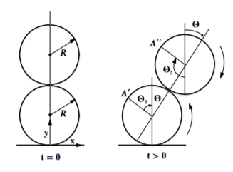
3. A uniform solid cylinder of radius \(R\) and mass \(M\) rests on a horizontal plane and an identical cylinder rests on it touching along the top of the first cylinder with the axes of both cylinders parallel. The upper cylinder is given an infinitessimal displacement so that both cylinders roll without slipping in the directions shown by the arrows.
   1. Find Lagrangian for this system
   2. What are the constants of motion?
   3. Show that as long as the cylinders remain in contact then

      \[\dot{\theta}^{2}=\frac{12g\left( 1-\cos \theta \right) }{R\left( 17+4\cos \theta -4\cos ^{2}\theta \right) }\]

      

      Figure \(\PageIndex{1}\)

4. Consider a diatomic molecule which has a symmetry axis along the line through the center of the two atoms comprising the molecule. Consider that this molecule is rotating about an axis perpendicular to the symmetry axis and that there are no external forces acting on the molecule. Use Noether’s Theorem to answer the following questions:
   1. Is the total angular momentum conserved?
   2. Is the projection of the total angular momentum along a space-fixed \(z\) axis conserved?
   3. Is the projection of the angular momentum along the symmetry axis of the rotating molecule conserved?
   4. Is the projection of the angular momentum perpendicular to the rotating symmetry axis conserved?
5. A bead of mass \(m\) slides under gravity along a smooth wire bent in the shape of a parabola \(x^{2}=az\) in the vertical \((x,z)\) plane.
   1. What kind (holonomic, nonholonomic, scleronomic, rheonomic) of constraint acts on \(m\)?
   2. Set up Lagrange’s equation of motion for \(x\) with the constraint embedded.
   3. Set up Lagrange’s equations of motion for both \(x\) and \(z\) with the constraint adjoined and a Lagrangian multiplier \(% \lambda\) introduced.
   4. Show that the same equation of motion for \(x\) results from either of the methods used in part (b) or part (c).
   5. Express \(\lambda\) in terms of \(x\) and \(\dot{x}\)
   6. What are the \(x\) and \(z\) components of the force of constraint in terms of \(x\) and \(\dot{x}\) ?
6. Let the horizontal plane be the \(x-y\) plane. A bead of mass \(m\) is constrained to slide with speed \(v\) along a curve described by the function \(y=f(x)\). What force does the curve apply to the bead? (Ignore gravity)
7. Consider the Atwoods machine shown. The masses are \(4m\), \(5m\), and \(3m\). Let \(x\) and \(y\) be the heights of the right two masses relative to their initial positions.
   1. Solve this problem using the Euler-Lagrange equations b) Use Noether’s theorem to find the conserved momentum.
   2. Use Noether’s theorem to find the conserved momentum.

      

      Figure \(\PageIndex{2}\)

8. A cube of side \(2b\) and center of mass \(C\), is placed on a fixed horizontal cylinder of radius \(r\) and center \(O\) as shown in the figure. Originally the cube is placed such that \(C\) is centered above \(O\) but it can roll from side to side without slipping. (a) Assuming that \(b<r\) use the Lagrangian approach to to find the frequency for small oscillations about the top of the cylinder. For simplicity make the small angle approximation for \(L\) before using the Lagrange-Euler equations. (b) What will be the motion if \(b>r\) ? Note that the moment of inertia of the cube about the center of mass is \(\frac{2}{3}mb^{2}\).

   

   Figure \(\PageIndex{3}\)

9. Two equal masses of mass \(m\) are glued to a massless hoop of radius \(R\) is free to rotate about its center in a vertical plane. The angle between the masses is \(2\theta\), as shown. Find the frequency of oscillations.

   

   Figure \(\PageIndex{4}\)

10. Three massless sticks each of length \(2r\), and mass \(% m\) with the center of mass at the center of each stick, are hinged at their ends as shown. The bottom end of the lower stick is hinged at the ground. They are held so that the lower two sticks are vertical, and the upper one is tilted at a small angle \(\varepsilon\) with respect to the vertical. They are then released. At the instant of release what are the three equations of motion derived from the Lagrangian derived assuming that \(\varepsilon\) is small\(?\) Use these to determine the initial angular accelerations of the three sticks.

    

    Figure \(\PageIndex{5}\)