
14.11: Damped Coupled Linear Oscillators
- Page ID
- 14258

The discussion of coupled linear oscillators has neglected non-conservative damping forces which always exist to some extent in physical systems. In general, dissipative forces are non linear which greatly complicates solving the equations of motion for such coupled oscillator systems. However, for some systems the dissipative forces depend linearly on velocity which allows use of the Rayleigh dissipation function, described in chapter \(10.4\). The most general definition of the Rayleigh dissipation function, \(10.4\), was given to be
\[\mathcal{R} = \frac{1}{2} \sum^n_{i=1} \sum^n_{j=1} c_{ij} \dot{q}_i\dot{q}_j \]
For this special case, it was shown in chapter \(10\) that the Lagrange equations can be written in terms of the Rayleigh dissipation function as
\[\left\{ \frac{d}{dt} \left( \frac{\partial L}{\partial \dot{q}_j}\right) - \frac{\partial L}{\partial q_j} \right\} + \frac{\partial \mathcal{R}}{\partial \dot{q}_j} = Q_j \label{14.120}\]
where \(Q_j\) are generalized forces acting on the system that are not absorbed into the potential \(U\). Using equations \((14.6.17)\), \((14.6.18)\), and \ref{14.120}, allows the equations of motion for damped coupled linear oscillators to be written in a matrix form as
\[\mathbf{\{T\}} \mathbf{\ddot{q}} + \mathbf{\{C\}} \mathbf{\dot{q}}+ \mathbf{\{V\}} \mathbf{q} = \mathbf{\{Q\}} \]
where the symmetric matrices \(\mathbf{\{T\}}\), \(\mathbf{\{C\}}\), and \(\mathbf{\{V\}}\) are positive definite for positive definite systems. Rayleigh pointed out that in the special case where the damping matrix \(\mathbf{\{C\}}\) is a linear combination of the \(\mathbf{\{T\}}\) and \(\mathbf{\{V\}}\) matrices, then the matrix \(\mathbf{\{C\}}\) is diagonal leading to a separation of the damped system into normal modes. As discussed in chapter 4 many systems in nature are linear for small amplitude oscillations allowing use of the Rayleigh dissipation function which provides an analytic solution. However, in general, except for when \(\mathbf{\{C\}}\) is small, this separation into normal modes is not possible for damped systems and the solutions must be obtained numerically.
The following example illustrates approaches used to handle linearly-damped coupled-oscillator systems.
Example \(\PageIndex{1}\): Two linearly-damped coupled linear oscillators
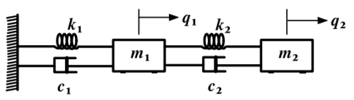
Consider the two coupled oscillator system shown where the two carts have spring constants \(k_1, k_2\) and linear damping constants \(c_1c_2\). As discussed in example \(14.7.2\), the kinetic energy tensor is given by
\[T = \frac{1}{2} m_1 \dot{q}^2_1 + \frac{1}{2} m_2 \dot{q}^{2}_{2} \label{a}\tag{a}\]
and the potential energy is given by
\[U = \frac{1}{2} \left[ k_1q^2_1 + k_2 (q_2 − q_1)^2 \right] \\ = \frac{1}{2} \left[ (k_1 + k_2) q^2_1 − 2k_2q_1q_2 + k_2q_2^2 \right] \label{b}\tag{b}\]
Similarly the Rayleigh dissipation function has the form
\[\mathcal{R} =\frac{1}{2} \left[ c_1\dot{q}^2_1 + c_2 ( \dot{q}^2_2 − \dot{q}^2_1 )\right] = \frac{1}{2} \left[ (c_1 + c_2) \dot{q}^2_1 − 2c_2\dot{q}_1\dot{q}_2 + c_2\dot{q}^2_2 \right] \label{c}\tag{c}\]
Inserting equations \ref{a}, \ref{b}, and \ref{c} into Equation \ref{14.120} gives the two equations of motion to be
\[m_1 \ddot{q}_1 + (c_1 + c_2) \dot{q}_1 − c_2\dot{q}_2 + (k_1 + k_2) q_1 − k_2q_2 = 0 \\ m_2 \ddot{q}_2 − c_2\dot{q}_1 + c_2\dot{q}_2 − k_2q_1 + k_2q_2 = 0 \nonumber\]
When the drag is zero the solution of these two coupled equations can be separated into two independent normal modes of the system as described earlier. Usually it is not possible to separate the motion into decoupled normal modes except for certain cases where the dissipative forces can be described by Rayleigh’s dissipation function.