
02. Drawing Motion Diagrams in 1D
- Page ID
- 582

\( \newcommand{\vecs}[1]{\overset { \scriptstyle \rightharpoonup} {\mathbf{#1}} } \)
\( \newcommand{\vecd}[1]{\overset{-\!-\!\rightharpoonup}{\vphantom{a}\smash {#1}}} \)
\( \newcommand{\id}{\mathrm{id}}\) \( \newcommand{\Span}{\mathrm{span}}\)
( \newcommand{\kernel}{\mathrm{null}\,}\) \( \newcommand{\range}{\mathrm{range}\,}\)
\( \newcommand{\RealPart}{\mathrm{Re}}\) \( \newcommand{\ImaginaryPart}{\mathrm{Im}}\)
\( \newcommand{\Argument}{\mathrm{Arg}}\) \( \newcommand{\norm}[1]{\| #1 \|}\)
\( \newcommand{\inner}[2]{\langle #1, #2 \rangle}\)
\( \newcommand{\Span}{\mathrm{span}}\)
\( \newcommand{\id}{\mathrm{id}}\)
\( \newcommand{\Span}{\mathrm{span}}\)
\( \newcommand{\kernel}{\mathrm{null}\,}\)
\( \newcommand{\range}{\mathrm{range}\,}\)
\( \newcommand{\RealPart}{\mathrm{Re}}\)
\( \newcommand{\ImaginaryPart}{\mathrm{Im}}\)
\( \newcommand{\Argument}{\mathrm{Arg}}\)
\( \newcommand{\norm}[1]{\| #1 \|}\)
\( \newcommand{\inner}[2]{\langle #1, #2 \rangle}\)
\( \newcommand{\Span}{\mathrm{span}}\) \( \newcommand{\AA}{\unicode[.8,0]{x212B}}\)
\( \newcommand{\vectorA}[1]{\vec{#1}} % arrow\)
\( \newcommand{\vectorAt}[1]{\vec{\text{#1}}} % arrow\)
\( \newcommand{\vectorB}[1]{\overset { \scriptstyle \rightharpoonup} {\mathbf{#1}} } \)
\( \newcommand{\vectorC}[1]{\textbf{#1}} \)
\( \newcommand{\vectorD}[1]{\overrightarrow{#1}} \)
\( \newcommand{\vectorDt}[1]{\overrightarrow{\text{#1}}} \)
\( \newcommand{\vectE}[1]{\overset{-\!-\!\rightharpoonup}{\vphantom{a}\smash{\mathbf {#1}}}} \)
\( \newcommand{\vecs}[1]{\overset { \scriptstyle \rightharpoonup} {\mathbf{#1}} } \)
\( \newcommand{\vecd}[1]{\overset{-\!-\!\rightharpoonup}{\vphantom{a}\smash {#1}}} \)
\(\newcommand{\avec}{\mathbf a}\) \(\newcommand{\bvec}{\mathbf b}\) \(\newcommand{\cvec}{\mathbf c}\) \(\newcommand{\dvec}{\mathbf d}\) \(\newcommand{\dtil}{\widetilde{\mathbf d}}\) \(\newcommand{\evec}{\mathbf e}\) \(\newcommand{\fvec}{\mathbf f}\) \(\newcommand{\nvec}{\mathbf n}\) \(\newcommand{\pvec}{\mathbf p}\) \(\newcommand{\qvec}{\mathbf q}\) \(\newcommand{\svec}{\mathbf s}\) \(\newcommand{\tvec}{\mathbf t}\) \(\newcommand{\uvec}{\mathbf u}\) \(\newcommand{\vvec}{\mathbf v}\) \(\newcommand{\wvec}{\mathbf w}\) \(\newcommand{\xvec}{\mathbf x}\) \(\newcommand{\yvec}{\mathbf y}\) \(\newcommand{\zvec}{\mathbf z}\) \(\newcommand{\rvec}{\mathbf r}\) \(\newcommand{\mvec}{\mathbf m}\) \(\newcommand{\zerovec}{\mathbf 0}\) \(\newcommand{\onevec}{\mathbf 1}\) \(\newcommand{\real}{\mathbb R}\) \(\newcommand{\twovec}[2]{\left[\begin{array}{r}#1 \\ #2 \end{array}\right]}\) \(\newcommand{\ctwovec}[2]{\left[\begin{array}{c}#1 \\ #2 \end{array}\right]}\) \(\newcommand{\threevec}[3]{\left[\begin{array}{r}#1 \\ #2 \\ #3 \end{array}\right]}\) \(\newcommand{\cthreevec}[3]{\left[\begin{array}{c}#1 \\ #2 \\ #3 \end{array}\right]}\) \(\newcommand{\fourvec}[4]{\left[\begin{array}{r}#1 \\ #2 \\ #3 \\ #4 \end{array}\right]}\) \(\newcommand{\cfourvec}[4]{\left[\begin{array}{c}#1 \\ #2 \\ #3 \\ #4 \end{array}\right]}\) \(\newcommand{\fivevec}[5]{\left[\begin{array}{r}#1 \\ #2 \\ #3 \\ #4 \\ #5 \\ \end{array}\right]}\) \(\newcommand{\cfivevec}[5]{\left[\begin{array}{c}#1 \\ #2 \\ #3 \\ #4 \\ #5 \\ \end{array}\right]}\) \(\newcommand{\mattwo}[4]{\left[\begin{array}{rr}#1 \amp #2 \\ #3 \amp #4 \\ \end{array}\right]}\) \(\newcommand{\laspan}[1]{\text{Span}\{#1\}}\) \(\newcommand{\bcal}{\cal B}\) \(\newcommand{\ccal}{\cal C}\) \(\newcommand{\scal}{\cal S}\) \(\newcommand{\wcal}{\cal W}\) \(\newcommand{\ecal}{\cal E}\) \(\newcommand{\coords}[2]{\left\{#1\right\}_{#2}}\) \(\newcommand{\gray}[1]{\color{gray}{#1}}\) \(\newcommand{\lgray}[1]{\color{lightgray}{#1}}\) \(\newcommand{\rank}{\operatorname{rank}}\) \(\newcommand{\row}{\text{Row}}\) \(\newcommand{\col}{\text{Col}}\) \(\renewcommand{\row}{\text{Row}}\) \(\newcommand{\nul}{\text{Nul}}\) \(\newcommand{\var}{\text{Var}}\) \(\newcommand{\corr}{\text{corr}}\) \(\newcommand{\len}[1]{\left|#1\right|}\) \(\newcommand{\bbar}{\overline{\bvec}}\) \(\newcommand{\bhat}{\widehat{\bvec}}\) \(\newcommand{\bperp}{\bvec^\perp}\) \(\newcommand{\xhat}{\widehat{\xvec}}\) \(\newcommand{\vhat}{\widehat{\vvec}}\) \(\newcommand{\uhat}{\widehat{\uvec}}\) \(\newcommand{\what}{\widehat{\wvec}}\) \(\newcommand{\Sighat}{\widehat{\Sigma}}\) \(\newcommand{\lt}{<}\) \(\newcommand{\gt}{>}\) \(\newcommand{\amp}{&}\) \(\definecolor{fillinmathshade}{gray}{0.9}\)Drawing Motion Diagrams (Qualitative)
The words used by physicists to describe the motion of objects are defined above. However, learning to use these terms correctly is more difficult than simply memorizing definitions. An extremely useful tool for bridging the gap between a normal, conversational description of a situation and a physicists’ description is the motion diagram. A motion diagram is the first step in translating a verbal description of a phenomenon into a physicists’ description.
Start with the following verbal description of a physical situation:
The driver of an automobile traveling at 15 m/s, noticing a red-light 30 m ahead, applies the brakes of her car until she stops just short of the intersection.
Determining the position from a motion diagram
A motion diagram can be thought of as a multiple-exposure photograph of the physical situation, with the image of the object exposed onto the film at equal time intervals. (You may have seen photographs of this type taken with a strobe-light.) For example, a multiple-exposure photograph of the situation described above would look something like this:
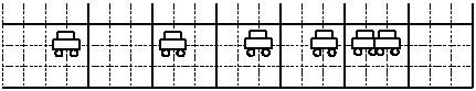
Note that the images of the automobile are getting closer together near the end of its motion because the car is traveling a smaller distance between the equally-timed exposures.
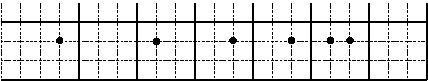
In general, in drawing motion diagrams it is better to represent the object as simply a dot, unless the actual shape of the object conveys some interesting information. Thus, a better motion diagram would be:
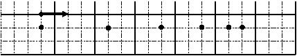
Since the purpose of the motion diagram is to help us describe the car’s motion, a coordinate system is necessary. Remember, to define a coordinate system you must choose a zero, define a positive direction, and select a scale. We will always use meters as our position scale in this course, so you must only select a zero and a positive direction. Remember, there is no correct answer. Any coordinate system is as correct as any other.
The choice below indicates that the initial position of the car is the origin, and positions to the right of that are positive.
We can now describe the position of the car. The car starts at position zero and then has positive, increasing positions throughout the remainder of its motion.
Determining the velocity from a motion diagram
Since velocity is the change in position of the car during a corresponding time interval, and we are free to select the time interval as the time interval between exposures on our multiple-exposure photograph, the velocity is simply the change in the position of the car "between dots." Thus, the arrows (vectors) on the motion diagram below represent the velocity of the car.
We can now describe the velocity of the car. Since the velocity vectors always point in the positive direction, the velocity is always positive. The car starts with a large, positive velocity which gradually declines until the velocity of the car is zero at the end of its motion.
Determining the acceleration from a motion diagram
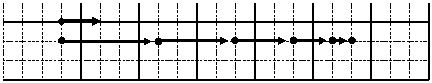
Since acceleration is the change in velocity of the car during a corresponding time interval, and we are free to select the time interval as the time interval between exposures on our multiple-exposure photograph, we can determine the acceleration by comparing two successive velocities. The change in these velocity vectors will represent the acceleration.
To determine the acceleration,
- select two successive velocity vectors,
- draw them starting from the same point,
- construct the vector (arrow) that connects the tip of the first velocity vector to the tip of the second velocity vector.
- The vector you have constructed represents the acceleration.
Comparing the first and second velocity vectors leads to the acceleration vector shown below:
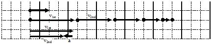
Thus, the acceleration points to the left and is therefore negative. You could construct the acceleration vector at every point in time, but hopefully you can see that as long as the velocity vectors continue to point toward the right and decrease in magnitude, the acceleration will remain negative.
Thus, with the help of a motion diagram, you can extract lots of information about the position, velocity, and acceleration of an object. You are well on your way to a complete kinematic description.