28.3: Length Contraction

Learning Objectives

By the end of this section, you will be able to:

• Describe proper length.
• Calculate length contraction.
• Explain why we don’t notice these effects at everyday scales.

Have you ever driven on a road that seems like it goes on forever? If you look ahead, you might say you have about 10 km left to go. Another traveler might say the road ahead looks like it’s about 15 km long. If you both measured the road, however, you would agree. Traveling at everyday speeds, the distance you both measure would be the same. You will read in this section, however, that this is not true at relativistic speeds. Close to the speed of light, distances measured are not the same when measured by different observers.

Figure \(\PageIndex{1}\): People might describe distances differently, but at relativistic speeds, the distances really are different. (credit: Corey Leopold, Flickr)

Proper Length

One thing all observers agree upon is relative speed. Even though clocks measure different elapsed times for the same process, they still agree that relative speed, which is distance divided by elapsed time, is the same. This implies that distance, too, depends on the observer’s relative motion. If two observers see different times, then they must also see different distances for relative speed to be the same to each of them.

The muon illustrates this concept. To an observer on the Earth, the muon travels at \(0.950c\) for \(7.05 \mu s\) from the time it is produced until it decays. Thus it travels a distance \[L_{0} = v \Delta t = \left(0.950\right)\left(3.00 \times 10^{8} m/s\right)\left(7.05 \times 10^{-6} s\right) = 2.01 km \label{28.4.1}\] relative to the Earth. In the muon’s frame of reference, its lifetime is only \(2.20 \mu s\). It has enough time to travel only \[L = v \Delta t_{0} = \left(0.950\right)\left(3.00 \times 10^{8} m/s\right)\left(2.20 \times 10^{-6} s\right) = 0.627 km. \label{28.4.2}\] The distance between the same two events (production and decay of a muon) depends on who measures it and how they are moving relative to it.

PROPER LENGTH

Proper length \(L_{0}\) is the distance between two points measured by an observer who is at rest relative to both of the points.

The Earth-bound observer measures the proper length \(L_{0}\), because the points at which the muon is produced and decays are stationary relative to the Earth. To the muon, the Earth, air, and clouds are moving, and so the distance \(L\) it sees is not the proper length.

Figure \(\PageIndex{2}\): (a) The Earth-bound observer sees the muon travel 2.01 km between clouds. (b) The muon sees itself travel the same path, but only a distance of 0.627 km. The Earth, air, and clouds are moving relative to the muon in its frame, and all appear to have smaller lengths along the direction of travel.

Length Contraction

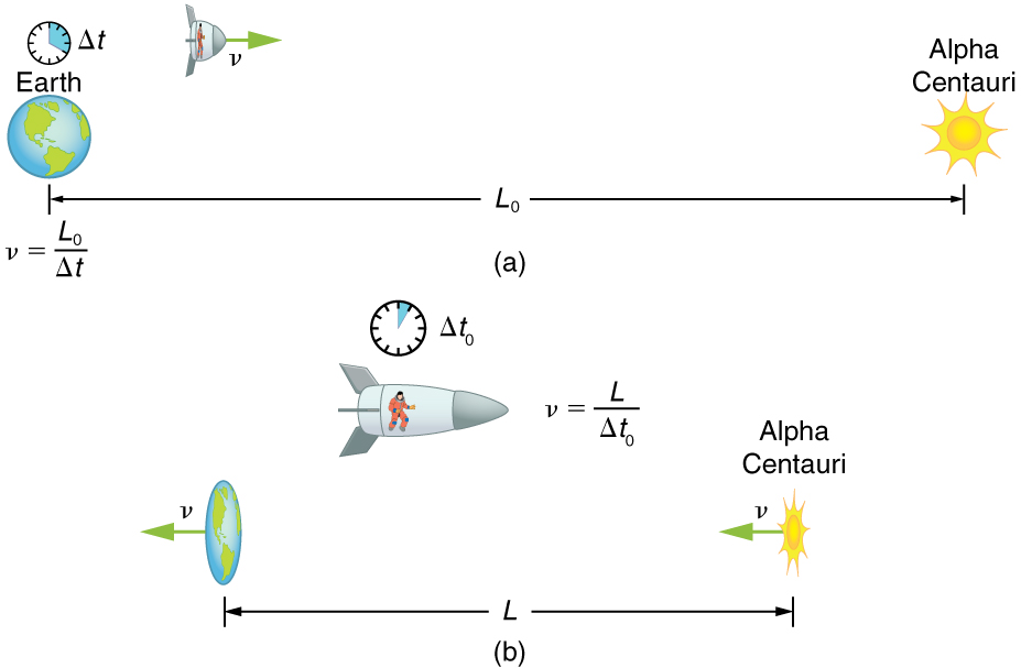
To develop an equation relating distances measured by different observers, we note that the velocity relative to the Earth-bound observer in our muon example is given by \[v = \frac{L_{0}}{\Delta t}.\label{28.4.3}\] The time relative to the Earth-bound observer is \(\Delta t\), since the object being timed is moving relative to this observer. The velocity relative to the moving observer is given by \[v = \frac{L}{\Delta t_{0}}.\label{28.4.4}\] The moving observer travels with the muon and therefore observes the proper time \(\Delta t_{0}\). The two velocities are identical; thus, \[\frac{L_{0}}{\Delta t} = \frac{L}{\Delta t_{0}}.\label{28..4.5}\] We know that \(\Delta t = \gamma \Delta t_{0}\). Substituting this equation into the relationship above gives \[L = \frac{L_{0}}{\gamma}.\label{28.4.6}\] Substituting for \(\gamma\) gives an equation relating the distances measured by different observers.

LENGTH CONTRACTION

Length contraction \(L\) is the shortening of the measured length of an object moving relative to the observer’s frame. \[L = L_{0} \sqrt{1-\frac{v^{2}}{c^{2}}}.\label{28.4.7}\]

If we measure the length of anything moving relative to our frame, we find its length \(L\) to be smaller than the proper length \(L_{0}\) that would be measured if the object were stationary. For example, in the muon’s reference frame, the distance between the points where it was produced and where it decayed is shorter. Those points are fixed relative to the Earth but moving relative to the muon. Clouds and other objects are also contracted along the direction of motion in the muon’s reference frame.

Example \(\PageIndex{1}\): Calculating Length Contraction: The Distance between Stars Contracts when You Travel at High Velocity:

Suppose an astronaut, such as the twin discussed in "Simultaneity and Time Dilation," travels so fast that \(\gamma = 30.00\). (a) She travels from the Earth to the nearest star system, Alpha Centauri, 4.300 light years (ly) away as measured by an Earth-bound observer. How far apart are the Earth and Alpha Centauri as measured by the astronaut? (b) In terms of \(c\), what is her velocity relative to the Earth? You may neglect the motion of the Earth relative to the Sun. (See Figure 3.)

Figure \(\PageIndex{3}\): (a) The Earth-bound observer measures the proper distance between the Earth and the Alpha Centauri. (b) The astronaut observes a length contraction, since the Earth and the Alpha Centauri move relative to her ship. She can travel this shorter distance in a smaller time (her proper time) without exceeding the speed of light.

Strategy

First note that a light year (ly) is a convenient unit of distance on an astronomical scale—it is the distance light travels in a year. For part (a), note that the 4.300 ly distance between the Alpha Centauri and the Earth is the proper distance \(l_0\), because it is measured by an Earth-bound observer to whom both stars are (approximately) stationary. To the astronaut, the Earth and the Alpha Centauri are moving by at the same velocity, and so the distance between them is the contracted length \(L\). In part (b), we are given \(\gamma\), and so we can find \(v\) by rearranging the definition of \(\gamma\) to express \(v\) in terms of \(c\).

Solution for (a)

1. Identify the knowns: \(L_0 - 4.300 \, ly; \, \gamma = 30.00\)
2. Identify the unknown: \(L\)
3. Choose the appropriate equation: \(L = \frac{L_0}{\gamma}\)
4. Rearrange the equation to solve for the unknown; \[L = \dfrac{L_0}{\gamma}\] \[= \dfrac{4.300 \, ly}{30.00}\] \[= 0.1433 \, ly\]

Solution for (b)

1. Identify the known: \(\gamma = 30.00\)
2. Identify the unknown: \(v\) in terms of \(c\)
3. Choose the appropriate equation \(\gamma = \frac{1}{\sqrt{1 - \frac{v^2}{c^2}}}\)
4. Rearrange the equation to solve for the unknown: \[\gamma = \dfrac{1}{\sqrt{1 - \frac{v^2}{c^2}}}\] \[ 30.00 = \dfrac{1}{\sqrt{1 - \frac{v^2}{c^2}}}\]

Squaring both sides of the equation and rearranging terms gives: \[900.0 = \dfrac{1}{1 - \frac{v^2}{c^2}}\]

so that \[1 - \dfrac{v^2}{c^2} = \dfrac{1}{900.0}\] and \[\dfrac{v^2}{c^2} = 1 - \dfrac{1}{900.0} = 0.99888....\]

Taking the square root, we find \[\dfrac{v}{c} = 0.99944,\] which is rearranged to produce a value for the velocity \[v = 0.9994c.\]

Discussion

First, remember that you should not round off calculations until the final result is obtained, or you could get erroneous results. This is especially true for special relativity calculations, where the differences might only be revealed after several decimal places. The relativistic effect is large here (γ=30.00), and we see that is approaching (not equaling) the speed of light. Since the distance as measured by the astronaut is so much smaller, the astronaut can travel it in much less time in her frame.

People could be sent very large distances (thousands or even millions of light years) and age only a few years on the way if they traveled at extremely high velocities. But, like emigrants of centuries past, they would leave the Earth they know forever. Even if they returned, thousands to millions of years would have passed on the Earth, obliterating most of what now exists. There is also a more serious practical obstacle to traveling at such velocities; immensely greater energies than classical physics predicts would be needed to achieve such high velocities. This will be discussed in Relatavistic Energy.

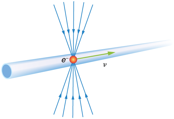
Why don’t we notice length contraction in everyday life? The distance to the grocery shop does not seem to depend on whether we are moving or not. Examining the equation \(L = L_0\sqrt{1 - \frac{v^2}{c^2}}\), we see that at low velocities \((v <<c)\) the lengths are nearly equal, the classical expectation. But length contraction is real, if not commonly experienced. For example, a charged particle, like an electron, traveling at relativistic velocity has electric field lines that are compressed along the direction of motion as seen by a stationary observer. (See Figure.) As the electron passes a detector, such as a coil of wire, its field interacts much more briefly, an effect observed at particle accelerators such as the 3 km long Stanford Linear Accelerator (SLAC). In fact, to an electron traveling down the beam pipe at SLAC, the accelerator and the Earth are all moving by and are length contracted. The relativistic effect is so great than the accelerator is only 0.5 m long to the electron. It is actually easier to get the electron beam down the pipe, since the beam does not have to be as precisely aimed to get down a short pipe as it would down one 3 km long. This, again, is an experimental verification of the Special Theory of Relativity.

Figure \(\PageIndex{41}\): The electric field lines of a high-velocity charged particle are compressed along the direction of motion by length contraction. This produces a different signal when the particle goes through a coil, an experimentally verified effect of length contraction.

Exercise \(\PageIndex{1}\)

A particle is traveling through the Earth’s atmosphere at a speed of \(0.750c\). To an Earth-bound observer, the distance it travels is 2.50 km. How far does the particle travel in the particle’s frame of reference?

Answer

\[L = L_0\sqrt{1 - \dfrac{v^2}{c^2}} = (2.50 \, km)\sqrt{1 - \dfrac{(0.750c)^2}{c^2}} = 1.65 \, km\]

Summary

• All observers agree upon relative speed.
• Distance depends on an observer’s motion. Proper length \(L_0\) is the distance between two points measured by an observer who is at rest relative to both of the points. Earth-bound observers measure proper length when measuring the distance between two points that are stationary relative to the Earth.
• Length contraction \(L\) is the shortening of the measured length of an object moving relative to the observer’s frame: \[L = L_0 \sqrt{1 - \dfrac{v^2}{c^2}} = \dfrac{L_0}{\gamma}.\]

Glossary

proper length

\(L_0\) the distance between two points measured by an observer who is at rest relative to both of the points; Earth-bound observers measure proper length when measuring the distance between two points that are stationary relative to the Earth

length contraction

\(L\) the shortening of the measured length of an object moving relative to the observer’s frame: \(L = L_0\sqrt{1 - \frac{v^2}{c^2}} = \frac{L_0}{\gamma}\)

Contributor

Paul Peter Urone (Professor Emeritus at California State University, Sacramento) and Roger Hinrichs (State University of New York, College at Oswego) with Contributing Authors: Kim Dirks (University of Auckland) and Manjula Sharma (University of Sydney). This work is licensed by OpenStax University Physics under a Creative Commons Attribution License (by 4.0).