8.9: Numerical Simulation of Skydiving Motion*

Last updated
Save as PDF

Page ID: 17775

$ \newcommand{\vecs}[1]{\overset { \scriptstyle \rightharpoonup} {\mathbf{#1}} } $ $ \newcommand{\vecd}[1]{\overset{-\!-\!\rightharpoonup}{\vphantom{a}\smash {#1}}} $$\newcommand{\id}{\mathrm{id}}$ $ \newcommand{\Span}{\mathrm{span}}$ $ \newcommand{\kernel}{\mathrm{null}\,}$ $ \newcommand{\range}{\mathrm{range}\,}$ $ \newcommand{\RealPart}{\mathrm{Re}}$ $ \newcommand{\ImaginaryPart}{\mathrm{Im}}$ $ \newcommand{\Argument}{\mathrm{Arg}}$ $ \newcommand{\norm}[1]{\| #1 \|}$ $ \newcommand{\inner}[2]{\langle #1, #2 \rangle}$ $ \newcommand{\Span}{\mathrm{span}}$ $\newcommand{\id}{\mathrm{id}}$ $ \newcommand{\Span}{\mathrm{span}}$ $ \newcommand{\kernel}{\mathrm{null}\,}$ $ \newcommand{\range}{\mathrm{range}\,}$ $ \newcommand{\RealPart}{\mathrm{Re}}$ $ \newcommand{\ImaginaryPart}{\mathrm{Im}}$ $ \newcommand{\Argument}{\mathrm{Arg}}$ $ \newcommand{\norm}[1]{\| #1 \|}$ $ \newcommand{\inner}[2]{\langle #1, #2 \rangle}$ $ \newcommand{\Span}{\mathrm{span}}$$\newcommand{\AA}{\unicode[.8,0]{x212B}}$

Our goal for this chapter is to graph the acceleration, velocity, and position of the skydiver from jump to terminal velocity, even though the acceleration changes throughout. We will use a numerical simulation that ties together just about everything we have learned so far in this unit to achieve this goal. We already know that the initial velocity is zero and because the drag force is zero when velocity is zero, the initial acceleration is g in the downward direction, or -9.8 m/s/s . We can then calculate the velocity after a short time interval quicklatex.com-f58525f7b6a89a5afea9ea67c672434f_l3.png as:

quicklatex.com-05954877165d8ada27c2c4487a092ec0_l3.png

We have made theassumption that the acceleration during this interval was constant, even though it wasn’t, but if we choose a time interval that is very small compared to the time over which the acceleration changes significantly, then our result is a good approximation. A time interval of 1 s will satisfy this condition in our case, so we now calculate the velocity at the end of the first short time interval:

quicklatex.com-12dc7690ef6011439931f4ded73c9e67_l3.png

Now that we have a velocity we can calculate the air resistance at the start of the second interval using our previous stated values for human drag coefficient, cross-sectional area, and the standard value for air density:

$s})^2 = 0.259 \,\bold{N} \end{equation*}$

Now that we have a drag force due to air resistance we can use Newton's Second Law to calculate the acceleration at the start of the second interval. We have only two forces, drag and gravity and we will use our previously stated skydiver mass of 80 kg:

$s} \end{equation*}$

Now we just continue this iterative process of using acceleration and velocity values from the previous interval to calculate new velocity, drag force, and acceleration for next interval.

Using the data produced by the simulation we can graph the drag force. Showing the weight on the same graph we can see how the drag force approaches the weight.

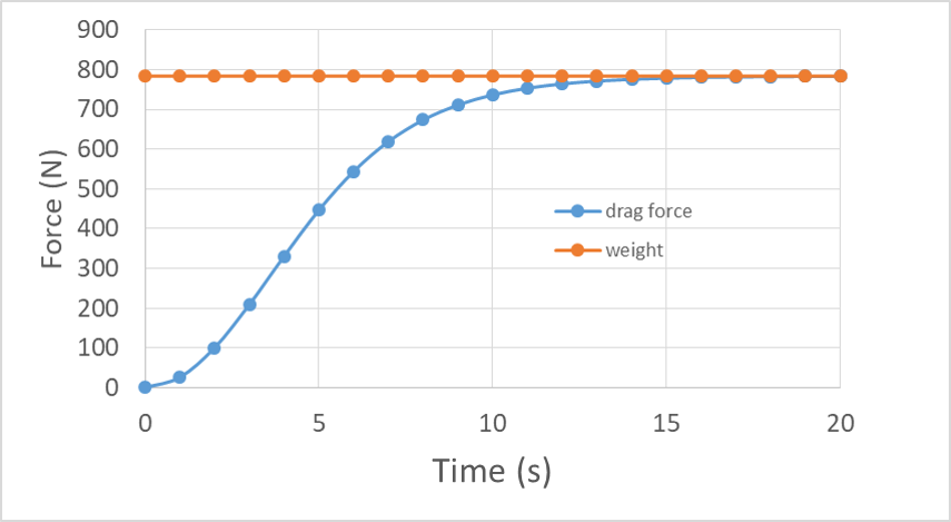
An example force vs. time curve for both drag and weight during a skydive. Weight is constant at 800 N. Drag starts at zero, increases with increasing slope (upward curvature), reaches an inflection point near 4 s, and continues to increase, but now with decreasing slope, and becomes indistinguishable from the weight value near 15 s.

We can also use the data to create motion graphs for the skydive and see that the acceleration gradually transitions from -9.8 m/s/s to zero as drag force increases.

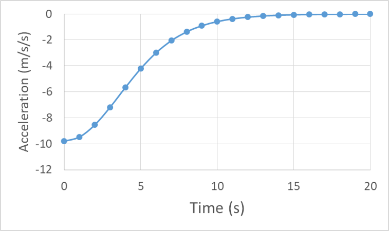
The acceleration vs. time curve replicates the shape of the force curve, but starts at -9.8 m/s/s, increases toward zero (slowing down) with increasing slope (upward curvature), reaches an inflection point near 4 s, and continues to increase, but now with decreasing slope, and becomes indistinguishable from zero near 15 s.

We see that velocity is always negative and the speed is always increasing, but the slope becomes less steep because the acceleration is decreasing with time:

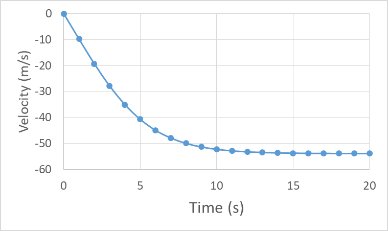
The velocity vs. time curve starts at zero and increases roughly linearly in the negative direction until near 4 s when it begins to level off and approach a constant 52 m/s.

Finally we can see that the position graph eventually becomes linear as terminal velocity is reached. (Note that we have converted our initial position of 12,000 ft to the equivalent 3660 m)

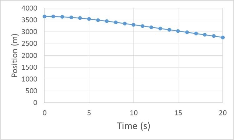
The position vs time curve starts at 3660 m and decreases toward zero with a negative and gradually steepening slope, nearing position 2750 m and slope of 52 m/s after 20 s.