3.5: Oscillations

Let's revisit the example of the stretched spring from the previous section. We know that its energy is a form of electrical energy of interacting atoms, which is nice conceptually but doesn't help us to solve problems, since we don't know how the energy, \(U\), depends on the length of the spring. All we know is that there's an equilibrium (figure a/1), which is a local minimum of the function \(U\). An extremely important problem which arises in this connection is how to calculate oscillatory motion around an equilibrium, as in a/4-13. Even if we did special experiments to find out how the spring's energy worked, it might seem like we'd have to go through just as much work to deal with any other kind of oscillation, such as a sapling swinging back and forth in the breeze.

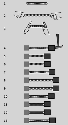
a / The spring has a minimum-energy length, 1, and energy is required in order to compress or stretch it, 2 and 3. A mass attached to the spring will oscillate around the equilibrium, 4-13.

Surprisingly, it's possible to analyze this type of oscillation in a very general and elegant manner, as long as the analysis is limited to small oscillations. We'll talk about the mass on the spring for concreteness, but there will be nothing in the discussion at all that is restricted to that particular physical system. First, let's choose a coordinate system in which \(x=0\) corresponds to the position of the mass where the spring is in equilibrium, and since interaction energies like \(U\) are only well defined up to an additive constant, we'll simply define it to be zero at equilibrium:

\[\begin{equation*} U(0) = 0 \end{equation*}\]

Since \(x=0\) is an equilibrium, \(U(x)\) must have a local minimum there, and a differentiable function (which we assume \(U\) is) has a zero derivative at a local minimum:

\[\begin{equation*} \frac{d{}U}{d{}x}(0) = 0 \end{equation*}\]

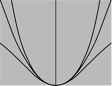
b / Three functions with the same curvature at \(x\)=0.

There are still infinitely many functions that could satisfy these criteria, including the three shown in figure b, which are \(x^2/2\), \(x^2/2(1+x^2)\), and \((e^{3x}+e^{-3x}-2)/18\). Note, however, how all three functions are virtually identical right near the minimum. That's because they all have the same curvature. More specifically, each function has its second derivative equal to 1 at \(x=0\), and the second derivative is a measure of curvature. We write \(k\) for the second derivative of the energy at an equilibrium point,

\[\begin{equation*} \frac{d{}^2U}{d{}x^2}(0) = k . \end{equation*}\]

Physically, \(k\) is a measure of stiffness. For example, the heavy-duty springs in a car's shock absorbers would have a high value of \(k\). It is often referred to as the spring constant, but we're only using a spring as an example here. As shown in figure b, any two functions that have \(U(0)=0\), \(d{}U/d{}x=0\), and \(d{}^2U/d{}x^2=k\), with the same value of \(k\), are virtually indistinguishable for small values of \(x\), so if we want to analyze small oscillations, it doesn't even matter which function we assume. For simplicity, we'll just use \(U(x)=(1/2)kx^2\) from now on.

Now we're ready to analyze the mass-on-a-spring system, while keeping in mind that it's really only a representative example of a whole class of similar oscillating systems. We expect that the motion is going to repeat itself over and over again, and since we're not going to include frictional heating in our model, that repetition should go on forever without dying out. The most interesting thing to know about the motion would be the period, \(T\), which is the amount of time required for one complete cycle of the motion. We might expect that the period would depend on the spring constant, \(k\), the mass, \(m\), and and the amplitude, \(A\), defined in figure c.¹¹

c / The amplitude would usually be defined as the distance from equilibrium to one extreme of the motion, i.e., half the total travel.

In examples like the brachistochrone and the Apollo 11 mission, it was generally necessary to use numerical techniques to determine the amount of time required for a certain motion. Once again, let's dust off the time3 function from page 93 and modify it for our purposes. For flexibility, we'll define the function \(U(x)\) as a separate Python function. We really want to calculate the time required for the mass to come back to its starting point, but that would be awkward to set up, since our function works by dividing up the distance to be traveled into tiny segments. By symmetry, the time required to go from one end to the other equals the time required to come back to the start, so we'll just calculate the time for half a cycle and then double it when we return the result at the end of the function. The test at lines 16-19 is necessary because otherwise at the very end of the motion we can end up trying to take the square root of a negative number due to rounding errors.

import math
def u(k,x):
  return .5*k*x**2

def osc(m,k,a,n):
  x=a
  v=0
  dx = -2.*a/n
  t=0
  e = u(k,x)+.5*m*v**2
  for i in range(n):
    x_old = x
    v_old = v
    x = x+dx
    kinetic = e-u(k,x)
    if kinetic<0. :
      v=0.
      print "warning, K=",kinetic,"<0"
    else :
      v = -math.sqrt(2.*kinetic/m)
    v_avg = (v+v_old)/2.
    dt=dx/v_avg
    t=t+dt
  return 2.*t

>>> print(osc(1.,1.,1.,100000))
warning, K= -1.43707268307e-12 <0
6.2831854132667919

The first thing to notice is that with this particular set of inputs (\(m\)=1 kg, \(k=1\ \text{J}/\text{m}^2\), and \(A=1\ \text{m}\)), the program has done an excellent job of computing \(2\pi=6.2831853...\). This is Mother Nature giving us a strong hint that the problem has an algebraic solution, not just a numerical one. The next interesting thing happens when we change the amplitude from 1 m to 2 m:

>>> print(osc(1.,1.,2.,100000))
warning, K= -5.7482907323e-12 <0
6.2831854132667919

Even though the mass had to travel double the distance in each direction, the period is the same to within the numerical accuracy of the calculation!

With these hints, it seems like we should start looking for an algebraic solution. For guidance, here's a graph of \(x\) as a function of \(t\), as calculated by the osc function with n=10.

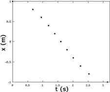
This looks like a cosine function, so let's see if a \(x=A\cos{}(\omega{}t+\delta)\) is a solution to the conservation of energy equation --- it's not uncommon to try to “reverse-engineer” the cryptic results of a numerical calculation like this. The symbol \(\omega=2\pi/T\) (Greek omega), called angular frequency, is a standard symbol for the number of radians per second of oscillation. Except for the factor of \(2\pi\), it is identical to the ordinary frequency \(f=1/T\), which has units of \(\text{s}^{-1}\) or Hz (Hertz). The phase angle \(\delta\) is to allow for the possibility that \(t=0\) doesn't coincide with the beginning of the motion. The energy is

\[\begin{align*} E &= K + U \\ &= \frac{1}{2}mv^2 + \frac{1}{2}kx^2 \\ &= \frac{1}{2}m\left(\frac{d{}x}{d{}t}\right)^2 + \frac{1}{2}kx^2 \\ &= \frac{1}{2}m\left[-A\omega\sin{}(\omega{}t+\delta)\right]^2 + \frac{1}{2}k\left[A\cos{}(\omega{}t+\delta)\right]^2 \\ &= \frac{1}{2}A^2\left[m\omega^2\sin{}^2(\omega{}t+\delta) + k\cos{}^2(\omega{}t+\delta)\right] \end{align*}\]

According to conservation of energy, this has to be a constant. Using the identity \(\sin^2+\cos^2=1\), we can see that it will be a constant if we have \(m\omega^2=k\), or \(\omega=\sqrt{k/m}\), i.e., \(T=2\pi\sqrt{m/k}\). Note that the period is independent of amplitude.

Example 23: A spring and a lever

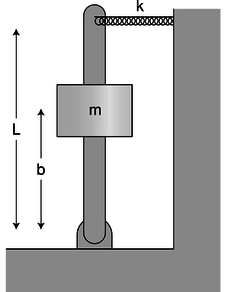
d / Example 23. The rod pivots on the hinge at the bottom. \(\triangleright\) What is the period of small oscillations of the system shown in the figure? Neglect the mass of the lever and the spring. Assume that the spring is so stiff that gravity is not an important effect. The spring is relaxed when the lever is vertical. \(\triangleright\) This is a little tricky, because the spring constant \(k\), although it is relevant, is not the \(k\) we should be putting into the equation \(T=2\pi\sqrt{m/k}\). The \(k\) that goes in there has to be the second derivative of \(U\) with respect to the position, \(x\), of the mass that's moving. The energy \(U\) stored in the spring depends on how far the tip of the lever is from the center. This distance equals \((L/b)x\), so the energy in the spring is \[\begin{align*} U &= \frac{1}{2}k\left(\frac{L}{b}x\right)^2 \\ &= \frac{kL^2}{2b^2}x^2 , \\ \end{align*}\] and the \(k\) we have to put in \(T=2\pi\sqrt{m/k}\) is \[\begin{equation*} \frac{d^2 U}{dx^2} = \frac{kL^2}{b^2} . \\ \end{equation*}\] The result is \[\begin{align*} T &= 2\pi\sqrt{\frac{mb^2}{kL^2}} \\ &= \frac{2\pi b}{L}\sqrt{\frac{m}{k}} \\ \end{align*}\] The leverage of the lever makes it as if the spring was stronger, and decreases the period of the oscillations by a factor of \(b/L\).

Example 24: Water in a U-shaped tube

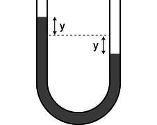
e / Water in a U-shaped tube. \(\triangleright\) What is the period of oscillation of the water in figure e? \(\triangleright\) In example 13 on p. 89, we found \(U( y)=\rho gAy^2\), so the “spring constant,” which really isn't a spring constant here at all, is \[\begin{align*} k &= \frac{\text{d}^2 U}{\text{d} y^2} \\ &= 2\rho gA . \end{align*}\] This is an interesting example, because \(k\) can be calculated without any approximations, but the kinetic energy requires an approximation, because we don't know the details of the pattern of flow of the water. It could be very complicated. There will be a tendency for the water near the walls to flow more slowly due to friction, and there may also be swirling, turbulent motion. However, if we make the approximation that all the water moves with the same velocity as the surface, \(\text{d} y/\text{d} t\), then the mass-on-a-spring analysis applies. Letting \(L\) be the total length of the filled part of the tube, the mass is \(\rho LA\), and we have \[\begin{align*} T &= 2\pi\sqrt{ m/ k} \\ &= 2\pi\sqrt{\frac{\rho LA}{2\rho gA}} \\ &= 2\pi\sqrt{\frac{ L}{2 g}} . \end{align*}\]

Contributors and Attributions

Benjamin Crowell (Fullerton College). Conceptual Physics is copyrighted with a CC-BY-SA license.