14.1: Rules of Randomness

• Given for one instant an intelligence which could comprehend all the forces by which nature is animated and the respective positions of the things which compose it...nothing would be uncertain, and the future as the past would be laid out before its eyes. -- Pierre Simon de Laplace, 1776
• The energy produced by the atom is a very poor kind of thing. Anyone who expects a source of power from the transformation of these atoms is talking moonshine. -- Ernest Rutherford, 1933
• The Quantum Mechanics is very imposing. But an inner voice tells me that it is still not the final truth. The theory yields much, but it hardly brings us nearer to the secret of the Old One. In any case, I am convinced that He does not play dice. -- Albert Einstein

However radical Newton's clockwork universe seemed to his contemporaries, by the early twentieth century it had become a sort of smugly accepted dogma. Luckily for us, this deterministic picture of the universe breaks down at the atomic level. The clearest demonstration that the laws of physics contain elements of randomness is in the behavior of radioactive atoms. Pick two identical atoms of a radioactive isotope, say the naturally occurring uranium 238, and watch them carefully. They will decay at different times, even though there was no difference in their initial behavior.

We would be in big trouble if these atoms' behavior was as predictable as expected in the Newtonian world-view, because radioactivity is an important source of heat for our planet. In reality, each atom chooses a random moment at which to release its energy, resulting in a nice steady heating effect. The earth would be a much colder planet if only sunlight heated it and not radioactivity. Probably there would be no volcanoes, and the oceans would never have been liquid. The deep-sea geothermal vents in which life first evolved would never have existed. But there would be an even worse consequence if radioactivity was deterministic: after a few billion years of peace, all the uranium 238 atoms in our planet would presumably pick the same moment to decay. The huge amount of stored nuclear energy, instead of being spread out over eons, would all be released at one instant, blowing our whole planet to Kingdom Come.¹

Figure \(\PageIndex{1}\): In 1980, the continental U.S. got its first taste of active volcanism in recent memory with the eruption of Mount St. Helens.

The new version of physics, incorporating certain kinds of randomness, is called quantum physics (for reasons that will become clear later). It represented such a dramatic break with the previous, deterministic tradition that everything that came before is considered “classical,” even the theory of relativity. This chapter is a basic introduction to quantum physics.

Exercise \(\PageIndex{1}\)

I said “Pick two identical atoms of a radioactive isotope.” Are two atoms really identical? If their electrons are orbiting the nucleus, can we distinguish each atom by the particular arrangement of its electrons at some instant in time?

Answer

Add texts here. Do not delete this text first.

13.1.1 Randomness isn't random

Einstein's distaste for randomness, and his association of determinism with divinity, goes back to the Enlightenment conception of the universe as a gigantic piece of clockwork that only had to be set in motion initially by the Builder. Many of the founders of quantum mechanics were interested in possible links between physics and Eastern and Western religious and philosophical thought, but every educated person has a different concept of religion and philosophy. Bertrand Russell remarked, “Sir Arthur Eddington deduces religion from the fact that atoms do not obey the laws of mathematics. Sir James Jeans deduces it from the fact that they do.”

Russell's witticism, which implies incorrectly that mathematics cannot describe randomness, remind us how important it is not to oversimplify this question of randomness. You should not simply surmise, “Well, it's all random, anything can happen.” For one thing, certain things simply cannot happen, either in classical physics or quantum physics. The conservation laws of mass, energy, momentum, and angular momentum are still valid, so for instance processes that create energy out of nothing are not just unlikely according to quantum physics, they are impossible.

A useful analogy can be made with the role of randomness in evolution. Darwin was not the first biologist to suggest that species changed over long periods of time. His two new fundamental ideas were that (1) the changes arose through random genetic variation, and (2) changes that enhanced the organism's ability to survive and reproduce would be preserved, while maladaptive changes would be eliminated by natural selection. Doubters of evolution often consider only the first point, about the randomness of natural variation, but not the second point, about the systematic action of natural selection. They make statements such as, “the development of a complex organism like Homo sapiens via random chance would be like a whirlwind blowing through a junkyard and spontaneously assembling a jumbo jet out of the scrap metal.” The flaw in this type of reasoning is that it ignores the deterministic constraints on the results of random processes. For an atom to violate conservation of energy is no more likely than the conquest of the world by chimpanzees next year.

Exercise \(\PageIndex{1}\)

Economists often behave like wannabe physicists, probably because it seems prestigious to make numerical calculations instead of talking about human relationships and organizations like other social scientists. Their striving to make economics work like Newtonian physics extends to a parallel use of mechanical metaphors, as in the concept of a market's supply and demand acting like a self-adjusting machine, and the idealization of people as economic automatons who consistently strive to maximize their own wealth. What evidence is there for randomness rather than mechanical determinism in economics?

Answer

Discussion Question - no answer given.

13.1.2 Calculating Randomness

You should also realize that even if something is random, we can still understand it, and we can still calculate probabilities numerically. In other words, physicists are good bookmakers. A good bookmaker can calculate the odds that a horse will win a race much more accurately that an inexperienced one, but nevertheless cannot predict what will happen in any particular race.

As an illustration of a general technique for calculating odds, suppose you are playing a 25-cent slot machine. Each of the three wheels has one chance in ten of coming up with a cherry. If all three wheels come up cherries, you win $100. Even though the results of any particular trial are random, you can make certain quantitative predictions. First, you can calculate that your odds of winning on any given trial are \(1/10\times1/10\times1/10=1/1000=0.001\). Here, I am representing the probabilities as numbers from 0 to 1, which is clearer than statements like “The odds are 999 to 1,” and makes the calculations easier. A probability of 0 represents something impossible, and a probability of 1 represents something that will definitely happen.

Also, you can say that any given trial is equally likely to result in a win, and it doesn't matter whether you have won or lost in prior games. Mathematically, we say that each trial is statistically independent, or that separate games are uncorrelated. Most gamblers are mistakenly convinced that, to the contrary, games of chance are correlated. If they have been playing a slot machine all day, they are convinced that it is “getting ready to pay,” and they do not want anyone else playing the machine and “using up” the jackpot that they “have coming.” In other words, they are claiming that a series of trials at the slot machine is negatively correlated, that losing now makes you more likely to win later. Craps players claim that you should go to a table where the person rolling the dice is “hot,” because she is likely to keep on rolling good numbers. Craps players, then, believe that rolls of the dice are positively correlated, that winning now makes you more likely to win later.

My method of calculating the probability of winning on the slot machine was an example of the following important rule for calculations based on independent probabilities:

The law of independent probabilities

If the probability of one event happening is \(P_A\), and the probability of a second statistically independent event happening is \(P_B\), then the probability that they will both occur is the product of the probabilities, \(P_AP_B\). If there are more than two events involved, you simply keep on multiplying.

This can be taken as the definition of statistical independence.

Note that this only applies to independent probabilities. For instance, if you have a nickel and a dime in your pocket, and you randomly pull one out, there is a probability of 0.5 that it will be the nickel. If you then replace the coin and again pull one out randomly, there is again a probability of 0.5 of coming up with the nickel, because the probabilities are independent. Thus, there is a probability of 0.25 that you will get the nickel both times.

Suppose instead that you do not replace the first coin before pulling out the second one. Then you are bound to pull out the other coin the second time, and there is no way you could pull the nickel out twice. In this situation, the two trials are not independent, because the result of the first trial has an effect on the second trial. The law of independent probabilities does not apply, and the probability of getting the nickel twice is zero, not 0.25.

Experiments have shown that in the case of radioactive decay, the probability that any nucleus will decay during a given time interval is unaffected by what is happening to the other nuclei, and is also unrelated to how long it has gone without decaying. The first observation makes sense, because nuclei are isolated from each other at the centers of their respective atoms, and therefore have no physical way of influencing each other. The second fact is also reasonable, since all atoms are identical. Suppose we wanted to believe that certain atoms were “extra tough,” as demonstrated by their history of going an unusually long time without decaying. Those atoms would have to be different in some physical way, but nobody has ever succeeded in detecting differences among atoms. There is no way for an atom to be changed by the experiences it has in its lifetime.

The Law of Independent Probabilities tells us to use multiplication to calculate the probability that both A and B will happen, assuming the probabilities are independent. What about the probability of an “or” rather than an “and”? If two events A and \(B\) are mutually exclusive, then the probability of one or the other occurring is the sum \(P_A+P_B\). For instance, a bowler might have a 30% chance of getting a strike (knocking down all ten pins) and a 20% chance of knocking down nine of them. The bowler's chance of knocking down either nine pins or ten pins is therefore 50%.

It does not make sense to add probabilities of things that are not mutually exclusive, i.e., that could both happen. Say I have a 90% chance of eating lunch on any given day, and a 90% chance of eating dinner. The probability that I will eat either lunch or dinner is not 180%.

Normalization

If I spin a globe and randomly pick a point on it, I have about a 70% chance of picking a point that's in an ocean and a 30% chance of picking a point on land. The probability of picking either water or land is \(70%+30%=100%\). Water and land are mutually exclusive, and there are no other possibilities, so the probabilities had to add up to 100%. It works the same if there are more than two possibilities --- if you can classify all possible outcomes into a list of mutually exclusive results, then all the probabilities have to add up to 1, or 100%. This property of probabilities is known as normalization.

Figure \(\PageIndex{2}\): Normalization: the probability of picking land plus the probability of picking water adds up to 1.

Averages

Another way of dealing with randomness is to take averages. The casino knows that in the long run, the number of times you win will approximately equal the number of times you play multiplied by the probability of winning. In the slot-machine game described on page 823, where the probability of winning is 0.001, if you spend a week playing, and pay $2500 to play 10,000 times, you are likely to win about 10 times \((10,000\times0.001=10)\), and collect $1000. On the average, the casino will make a profit of $1500 from you. This is an example of the following rule.

Rule for Calculating Averages

If you conduct \(N\) identical, statistically independent trials, and the probability of success in each trial is \(P\), then on the average, the total number of successful trials will be \(NP\). If \(N\) is large enough, the relative error in this estimate will become small.

The statement that the rule for calculating averages gets more and more accurate for larger and larger \(N\) (known popularly as the “law of averages”) often provides a correspondence principle that connects classical and quantum physics. For instance, the amount of power produced by a nuclear power plant is not random at any detectable level, because the number of atoms in the reactor is so large. In general, random behavior at the atomic level tends to average out when we consider large numbers of atoms, which is why physics seemed deterministic before physicists learned techniques for studying atoms individually.

We can achieve great precision with averages in quantum physics because we can use identical atoms to reproduce exactly the same situation many times. If we were betting on horses or dice, we would be much more limited in our precision. After a thousand races, the horse would be ready to retire. After a million rolls, the dice would be worn out.

Exercise \(\PageIndex{1}\)

Which of the following things must be independent, which could be independent, and which definitely are not independent? (1) the probability of successfully making two free-throws in a row in basketball; (2) the probability that it will rain in London tomorrow and the probability that it will rain on the same day in a certain city in a distant galaxy; (3) your probability of dying today and of dying tomorrow.

Answer

Answer in the back of the PDF version of the book.

Exercise \(\PageIndex{1}\) Discussion Questions

Figure \(\PageIndex{3}\): Why are dice random?

• Newtonian physics is an essentially perfect approximation for describing the motion of a pair of dice. If Newtonian physics is deterministic, why do we consider the result of rolling dice to be random?
• Why isn't it valid to define randomness by saying that randomness is when all the outcomes are equally likely?
• The sequence of digits 121212121212121212 seems clearly nonrandom, and 41592653589793 seems random. The latter sequence, however, is the decimal form of pi, starting with the third digit. There is a story about the Indian mathematician Ramanujan, a self-taught prodigy, that a friend came to visit him in a cab, and remarked that the number of the cab, 1729, seemed relatively uninteresting. Ramanujan replied that on the contrary, it was very interesting because it was the smallest number that could be represented in two different ways as the sum of two cubes. The Argentine author Jorge Luis Borges wrote a short story called “The Library of Babel,” in which he imagined a library containing every book that could possibly be written using the letters of the alphabet. It would include a book containing only the repeated letter “a;” all the ancient Greek tragedies known today, all the lost Greek tragedies, and millions of Greek tragedies that were never actually written; your own life story, and various incorrect versions of your own life story; and countless anthologies containing a short story called “The Library of Babel.” Of course, if you picked a book from the shelves of the library, it would almost certainly look like a nonsensical sequence of letters and punctuation, but it's always possible that the seemingly meaningless book would be a science-fiction screenplay written in the language of a Neanderthal tribe, or the lyrics to a set of incomparably beautiful love songs written in a language that never existed. In view of these examples, what does it really mean to say that something is random?

Answer

Add texts here. Do not delete this text first.

13.1.3 Probability Distributions

So far we've discussed random processes having only two possible outcomes: yes or no, win or lose, on or off. More generally, a random process could have a result that is a number. Some processes yield integers, as when you roll a die and get a result from one to six, but some are not restricted to whole numbers, for example the number of seconds that a uranium-238 atom will exist before undergoing radioactive decay.

Consider a throw of a die. If the die is “honest,” then we expect all six values to be equally likely. Since all six probabilities must add up to 1, then probability of any particular value coming up must be 1/6. We can summarize this in a graph (Figure \(\PageIndex{4a}\)). Areas under the curve can be interpreted as total probabilities. For instance, the area under the curve from 1 to 3 is \(1/6+1/6+1/6=1/2\), so the probability of getting a result from 1 to 3 is 1/2. The function shown on the graph is called the probability distribution.

Figure \(\PageIndex{4}\): (a)Probability distribution for the result of rolling a single die. (b) Rolling two dice and adding them up.

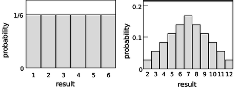
Figure \(\PageIndex{4b}\) shows the probabilities of various results obtained by rolling two dice and adding them together, as in the game of craps. The probabilities are not all the same. There is a small probability of getting a two, for example, because there is only one way to do it, by rolling a one and then another one. The probability of rolling a seven is high because there are six different ways to do it: 1+6, 2+5, etc.

If the number of possible outcomes is large but finite, for example the number of hairs on a dog, the graph would start to look like a smooth curve rather than a ziggurat.

What about probability distributions for random numbers that are not integers? We can no longer make a graph with probability on the \(y\) axis, because the probability of getting a given exact number is typically zero. For instance, there is zero probability that a radioactive atom will last for exactly 3 seconds, since there is are infinitely many possible results that are close to 3 but not exactly three: 2.999999999999999996876876587658465436, for example. It doesn't usually make sense, therefore, to talk about the probability of a single numerical result, but it does make sense to talk about the probability of a certain range of results. For instance, the probability that an atom will last more than 3 and less than 4 seconds is a perfectly reasonable thing to discuss. We can still summarize the probability information on a graph, and we can still interpret areas under the curve as probabilities.

But the \(y\) axis can no longer be a unitless probability scale. In radioactive decay, for example, we want the \(x\) axis to have units of time, and we want areas under the curve to be unitless probabilities. The area of a single square on the graph paper is then

\[\begin{gather*} \text{(unitless area of a square)} \\ = \text{(width of square with time units)}\\ \times \text{(height of square)} . \end{gather*}\]

If the units are to cancel out, then the height of the square must evidently be a quantity with units of inverse time. In other words, the \(y\) axis of the graph is to be interpreted as probability per unit time, not probability. Figure \(\PageIndex{5}\) shows another example, a probability distribution for people's height. This kind of bell-shaped curve is quite common.\

Figure \(\PageIndex{5}\): A probability distribution for height of human adults (not real data).

Exercise \(\PageIndex{1}\)

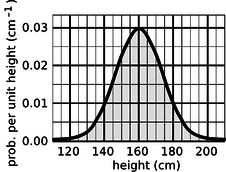
Compare the number of people with heights in the range of 130-135 cm to the number in the range 135-140

Answer

(answer in the back of the PDF version of the book).

Example \(\PageIndex{1}\): Looking for tall basketball players

A certain country with a large population wants to find very tall people to be on its Olympic basketball team and strike a blow against western imperialism. Out of a pool of \(10^8\) people who are the right age and gender, how many are they likely to find who are over 225 cm (7 feet 4 inches) in height? Figure g gives a close-up of the “tail” of the distribution shown previously in Figure \(\PageIndex{6}\).

Figure \(\PageIndex{6}\)

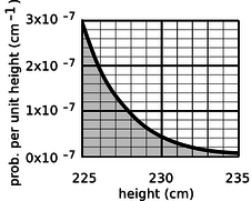
The shaded area under the curve represents the probability that a given person is tall enough. Each rectangle represents a probability of \(0.2\times10^{-7}\ \text{cm}^{-1} \times 1\ \text{cm}=2\times10^{-8}\). There are about 35 rectangles covered by the shaded area, so the probability of having a height greater than 225 cm is \(7\times10^{-7}\), or just under one in a million. Using the rule for calculating averages, the average, or expected number of people this tall is \((10^8)\times(7\times10^{-7})=70\).

Average and width of a probability distribution

If the next Martian you meet asks you, “How tall is an adult human?,” you will probably reply with a statement about the average human height, such as “Oh, about 5 feet 6 inches.” If you wanted to explain a little more, you could say, “But that's only an average. Most people are somewhere between 5 feet and 6 feet tall.” Without bothering to draw the relevant bell curve for your new extraterrestrial acquaintance, you've summarized the relevant information by giving an average and a typical range of variation.

Figure \(\PageIndex{6}\): The average of a probability distribution.

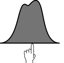
The average of a probability distribution can be defined geometrically as the horizontal position at which it could be balanced if it was constructed out of cardboard. A convenient numerical measure of the amount of variation about the average, or amount of uncertainty, is the full width at half maximum, or FWHM, shown in Figure \(\PageIndex{7}\).

Figure \(\PageIndex{7}\): The full width at half maximum (FWHM) of a probability distribution.

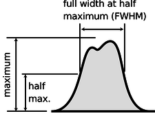
A great deal more could be said about this topic, and indeed an introductory statistics course could spend months on ways of defining the center and width of a distribution. Rather than force-feeding you on mathematical detail or techniques for calculating these things, it is perhaps more relevant to point out simply that there are various ways of defining them, and to inoculate you against the misuse of certain definitions.

The average is not the only possible way to say what is a typical value for a quantity that can vary randomly; another possible definition is the median, defined as the value that is exceeded with 50% probability. When discussing incomes of people living in a certain town, the average could be very misleading, since it can be affected massively if a single resident of the town is Bill Gates. Nor is the FWHM the only possible way of stating the amount of random variation; another possible way of measuring it is the standard deviation (defined as the square root of the average squared deviation from the average value).

13.1.4 Exponential Decay and Half-life

Most people know that radioactivity “lasts a certain amount of time,” but that simple statement leaves out a lot. As an example, consider the following medical procedure used to diagnose thyroid function. A very small quantity of the isotope \(^{131}\text{I}\), produced in a nuclear reactor, is fed to or injected into the patient. The body's biochemical systems treat this artificial, radioactive isotope exactly the same as \(^{127}\text{I}\), which is the only naturally occurring type. (Nutritionally, iodine is a necessary trace element. Iodine taken into the body is partly excreted, but the rest becomes concentrated in the thyroid gland. Iodized salt has had iodine added to it to prevent the nutritional deficiency known as goiters, in which the iodine-starved thyroid becomes swollen.) As the \(^{131}\text{I}\) undergoes beta decay, it emits electrons, neutrinos, and gamma rays. The gamma rays can be measured by a detector passed over the patient's body. As the radioactive iodine becomes concentrated in the thyroid, the amount of gamma radiation coming from the thyroid becomes greater, and that emitted by the rest of the body is reduced. The rate at which the iodine concentrates in the thyroid tells the doctor about the health of the thyroid.

If you ever undergo this procedure, someone will presumably explain a little about radioactivity to you, to allay your fears that you will turn into the Incredible Hulk, or that your next child will have an unusual number of limbs. Since iodine stays in your thyroid for a long time once it gets there, one thing you'll want to know is whether your thyroid is going to become radioactive forever. They may just tell you that the radioactivity “only lasts a certain amount of time,” but we can now carry out a quantitative derivation of how the radioactivity really will die out.

Let \(P_{surv}(t)\) be the probability that an iodine atom will survive without decaying for a period of at least \(t\). It has been experimentally measured that half all \(^{131}\text{I}\) atoms decay in 8 hours, so we have

\[ P_{surv}(8\ \text{hr}) = 0.5 . \]

Now using the law of independent probabilities, the probability of surviving for 16 hours equals the probability of surviving for the first 8 hours multiplied by the probability of surviving for the second 8 hours,

\[\begin{align*} P_{surv}(16\ \text{hr}) &= 0.50\times0.50 \\ &= 0.25 . \end{align*}\]

Similarly we have

\[\begin{align*} P_{surv}(24\ \text{hr}) &= 0.50\times0.5\times0.5 \\ &= 0.125 . \end{align*}\]

Generalizing from this pattern, the probability of surviving for any time \(t\) that is a multiple of 8 hours is

\[ P_{surv}(t) = 0.5^{t/8\ \text{hr}} . \]

We now know how to find the probability of survival at intervals of 8 hours, but what about the points in time in between? What would be the probability of surviving for 4 hours? Well, using the law of independent probabilities again, we have

\[ P_{surv}(8\ \text{hr}) = P_{surv}(4\ \text{hr}) \times P_{surv}(4\ \text{hr}) , \]

which can be rearranged to give

\[\begin{align*} P_{surv}(4\ \text{hr}) &= \sqrt{P_{surv}(8\ \text{hr})} \\ &= \sqrt{0.5} \\ &= 0.707 . \end{align*}\]

This is exactly what we would have found simply by plugging in \(P_{surv}(t)=0.5^{t/8\ \text{hr}}\) and ignoring the restriction to multiples of 8 hours. Since 8 hours is the amount of time required for half of the atoms to decay, it is known as the half-life, written \(t_{1/2}\). The general rule is as follows:

\[ \underbrace{P_{surv}(t) = 0.5^{t/t_{1/2}}}_{\text{Exponential Decay Equation}} \]

Using the rule for calculating averages, we can also find the number of atoms, \(N(t)\), remaining in a sample at time \(t \):

\[ N(t) = N(0) \times 0.5^{t/t_{1/2}} \]

Both of these equations have graphs that look like dying-out exponentials, as in the example below.

Example \(\PageIndex{2}\): Radioactive contamination at Chernobyl

One of the most dangerous radioactive isotopes released by the Chernobyl disaster in 1986 was \(^{90}\text{Sr}\), whose half-life is 28 years. (a) How long will it be before the contamination is reduced to one tenth of its original level? (b) If a total of \(10^{27}\) atoms was released, about how long would it be before not a single atom was left?

Solution

(a) We want to know the amount of time that a \(^{90}\text{Sr}\) nucleus has a probability of 0.1 of surviving. Starting with the exponential decay formula,

\[ P_{surv} = 0.5^{t/t_{1/2}} , \nonumber \]

we want to solve for \(t\). Taking natural logarithms of both sides,

\[ \ln P = \frac{t}{t_{1/2}}\ln 0.5 , \nonumber\]

so

\[ t = \frac{t_{1/2}}{\ln 0.5}\ln P \nonumber \]

Plugging in \(P=0.1\) and \(t_{1/2}=28\) years, we get \(t=93\) years.

(b) This is just like the first part, but \(P=10^{-27}\). The result is about 2500 years.

Example \(\PageIndex{3}\): \(^{14}\text{C}\) Dating

Almost all the carbon on Earth is \(^{12}\text{C}\), but not quite. The isotope \(^{14}\text{C}\), with a half-life of 5600 years, is produced by cosmic rays in the atmosphere. It decays naturally, but is replenished at such a rate that the fraction of \(^{14}\text{C}\) in the atmosphere remains constant, at \(1.3\times10^{-12}\). Living plants and animals take in both \(^{12}\text{C}\) and \(^{14}\text{C}\) from the atmosphere and incorporate both into their bodies. Once the living organism dies, it no longer takes in C atoms from the atmosphere, and the proportion of \(^{14}\text{C}\) gradually falls off as it undergoes radioactive decay. This effect can be used to find the age of dead organisms, or human artifacts made from plants or animals. Figure j shows the exponential decay curve of \(^{14}\text{C}\) in various objects. Similar methods, using longer-lived isotopes, provided the first firm proof that the earth was billions of years old, not a few thousand as some had claimed on religious grounds.

Figure \(\PageIndex{8}\): Calibration of the \(^{14}\text{C}\) dating method using tree rings and artifacts whose ages were known from other methods. Redrawn from Emilio Segrè, Nuclei and Particles, 1965.

Rate of Decay

If you want to find how many radioactive decays occur within a time interval lasting from time \(t\) to time \(t+\Delta t\), the most straightforward approach is to calculate it like this:

\[\begin{align*} (\text{number of}&\text{ decays between } t \text{ and } t+\Delta t) \\ &= N(t) - N(t+\Delta t) \end{align*}\]

Usually we're interested in the case where \(\Delta t\) is small compared to \(t_{1/2}\), and in this limiting case the calculation starts to look exactly like the limit that goes into the definition of the derivative \(dN/dt\). It is therefore more convenient to talk about the rate of decay \(-dN/dt\) rather than the number of decays in some finite time interval. Doing calculus on the function \(e^x\) is also easier than with \(0.5^x\), so we rewrite the function \(N(t)\) as

\[ N = N(0) e^{-t/\tau} , \]

where \(\tau=t_{1/2}/\ln 2\) is shown in example 6 on p. 835 to be the average time of survival. The rate of decay is then

\[ -\frac{dN}{dt} = \frac{N(0)}{\tau} e^{-t/\tau} . \]

Mathematically, differentating an exponential just gives back another exponential. Physically, this is telling us that as \(N\) falls off exponentially, the rate of decay falls off at the same exponential rate, because a lower \(N\) means fewer atoms that remain available to decay.

Exercise \(\PageIndex{1}\)

Check that both sides of the equation for the rate of decay have units of \(\text{s}^{-1}\), i.e., decays per unit time.

Answer

answer in the back of the PDF version of the book)

Example \(\PageIndex{4}\): The hot potato

A nuclear physicist with a demented sense of humor tosses you a cigar box, yelling “hot potato.” The label on the box says “contains \(10^{20}\) atoms of \(^{17}\text{F}\), half-life of 66 s, produced today in our reactor at 1 p.m.” It takes you two seconds to read the label, after which you toss it behind some lead bricks and run away. The time is 1:40 p.m. Will you die?

Solution

The time elapsed since the radioactive fluorine was produced in the reactor was 40 minutes, or 2400 s. The number of elapsed half-lives is therefore \(t/t_{1/2}= 36\). The initial number of atoms was \(N(0)=10^{20}\). The number of decays per second is now about \(10^7\ \text{s}^{-1}\), so it produced about \(2\times10^7\) high-energy electrons while you held it in your hands. Although twenty million electrons sounds like a lot, it is not really enough to be dangerous.

By the way, none of the equations we've derived so far was the actual probability distribution for the time at which a particular radioactive atom will decay. That probability distribution would be found by substituting \(N(0)=1\) into the equation for the rate of decay.

Discussion Questions

◊ In the medical procedure involving \(^{131}\text{I}\), why is it the gamma rays that are detected, not the electrons or neutrinos that are also emitted?

◊ For 1 s, Fred holds in his hands 1 kg of radioactive stuff with a half-life of 1000 years. Ginger holds 1 kg of a different substance, with a half-life of 1 min, for the same amount of time. Did they place themselves in equal danger, or not?

◊ How would you interpret it if you calculated \(N(t)\), and found it was less than one?

◊ Does the half-life depend on how much of the substance you have? Does the expected time until the sample decays completely depend on how much of the substance you have?

13.1.5 Applications of Calculus

The area under the probability distribution is of course an integral. If we call the random number \(x\) and the probability distribution \(D(x)\), then the probability that \(x\) lies in a certain range is given by

\[ \text{(probability of $a\le x \le b$)}=\int_a^b D(x) dx . \]

What about averages? If \(x\) had a finite number of equally probable values, we would simply add them up and divide by how many we had. If they weren't equally likely, we'd make the weighted average \(x_1P_1+x_2P_2+\)... But we need to generalize this to a variable \(x\) that can take on any of a continuum of values. The continuous version of a sum is an integral, so the average is

\[ \text{(average value of $x$)} = \int x D(x) dx , \]

where the integral is over all possible values of \(x\).

Example \(\PageIndex{5}\): Probability distribution for radioactive decay

Here is a rigorous justification for the statement in subsection 13.1.4 that the probability distribution for radioactive decay is found by substituting \(N(0)=1\) into the equation for the rate of decay. We know that the probability distribution must be of the form

\[ D(t) = k 0.5^{t/t_{1/2}} , \]

where \(k\) is a constant that we need to determine. The atom is guaranteed to decay eventually, so normalization gives us

\[\begin{align*} \text{(probability of $0\le t \lt \infty$)} &= 1 \\ &= \int_0^\infty D(t) dt . \end{align*}\]

The integral is most easily evaluated by converting the function into an exponential with \(e\) as the base

\[\begin{align*} D(t) &= k \exp\left[\ln\left(0.5^{t/t_{1/2}}\right)\right] \\ &= k \exp\left[\frac{t}{t_{1/2}}\ln 0.5\right] \\ &= k \exp\left(-\frac{\ln 2}{t_{1/2}}t\right) , \end{align*}\]

which gives an integral of the familiar form \(\int e^{cx}dx=(1/c)e^{cx}\). We thus have

\[ 1 = \left.-\frac{kt_{1/2}}{\ln 2}\exp\left(-\frac{\ln 2}{t_{1/2}}t\right)\right]_0^\infty , \]

which gives the desired result:

\[ k = \frac{\ln 2}{t_{1/2}} . \]

Example \(\PageIndex{6}\): Average lifetime

You might think that the half-life would also be the average lifetime of an atom, since half the atoms' lives are shorter and half longer. But the half whose lives are longer include some that survive for many half-lives, and these rare long-lived atoms skew the average. We can calculate the average lifetime as follows:

\[ (\text{average lifetime}) = \int_0^\infty t\: D(t)dt \]

Using the convenient base-\(e\) form again, we have

\[ (\text{average lifetime}) = \frac{\ln 2}{t_{1/2}} \int_0^\infty t \exp\left(-\frac{\ln 2}{t_{1/2}}t\right) dt . \]

This integral is of a form that can either be attacked with integration by parts or by looking it up in a table. The result is \(\int x e^{cx}dx=\frac{x}{c}e^{cx}-\frac{1}{c^2}e^{cx}\), and the first term can be ignored for our purposes because it equals zero at both limits of integration. We end up with

\[\begin{align*} \text{(average lifetime)} &= \frac{\ln 2}{t_{1/2}}\left(\frac{t_{1/2}}{\ln 2}\right)^2 \\ &= \frac{t_{1/2}}{\ln 2} \\ &= 1.443 \: t_{1/2} , \end{align*}\]

which is, as expected, longer than one half-life.

Figure \(\PageIndex{9}\): In recent decades, a huge hole in the ozone layer has spread out from Antarctica. Left: November 1978. Right: November 1992

Contributors and Attributions

• Benjamin Crowell (Fullerton College). Conceptual Physics is copyrighted with a CC-BY-SA license.