2.2: The Scalar Potential Function

The direct calculation of the electric field using Coulomb’s law as in Equation (2.1.5) is usually inconvenient because of the vector character of the electric field: Equation (2.1.5) is actually three equations, one for each electric field component \(\vec E\)_x, \(\vec E\)_y, and \(\vec E\)_z. It turns out that the electrostatic field can be obtained from a single scalar function, V(x,y,z), called the potential function. Usually it is easier to calculate the potential function than it is to calculate the electric field directly. The field \(\vec E\) can be obtained from the potential function by differentiation:

\[\overrightarrow{\mathrm{E}}(x, y, z)=-\operatorname{grad} V(x, y, z). \label{2.8}\]

That is in cartesian co-ordinates

\[ \begin{align} &E_{x}=-\frac{\partial V}{\partial x}, \nonumber \\& E_{y}=-\frac{\partial V}{\partial y}, \nonumber \\& E_{z}=-\frac{\partial V}{\partial z}. \nonumber \end{align} \nonumber \]

According to the Maxwell Equation (2.1.1) the curl(\(\vec E\)) must be zero for the electro-static field. This equation is automatically satisfied by Equation (2.2.1) because of the mathematical theorem that states that the curl of any gradient function is zero, see section (1.3.1). The units of the potential function are Volts. Absolute potential has no meaning. One can add or subtract a constant potential from the potential function without changing the electric field; the electric field is the physically meaningful quantity. Since the electric field satisfies the law of superposition it follows that the potential function must also satisfy superposition. This means that the potential function at any point due to a collection of charges must simply be the sum of the potentials generated at that point by each charge acting as if it were alone. One of the virtues of using a potential function is that scalar quantities are easier to add than are vector quantities because one has only to deal with one number at each point in space rather than the three numbers which specify a vector (the three components). Of course, to obtain the electric field from the potential function at some point in space it is necessary to know the potential at that point plus the value of the potential at nearby points in order to be able to calculate the derivatives in grad(V).

The electric field at the point \(\vec R\), whose co-ordinates are (X,Y,Z), due to a point charge q at \(\vec r\), whose co-ordinates are (x,y,z), can be calculated from the potential function

\[V(\overrightarrow{\mathrm{R}})=\frac{q}{4 \pi \epsilon_{0}} \frac{1}{|\overrightarrow{\mathrm{R}}-\overrightarrow{\mathrm{r}}|}, \label{2.9}\]

or

\[V(X, Y, Z)=\frac{q}{4 \pi \epsilon_{0}} \frac{1}{\left[(X-x)^{2}+(Y-y)^{2}+(Z-z)^{2}\right]^{1 / 2}}. \nonumber\]

That this is an appropriate potential function can be verified by direct differentiation using

\[ \begin{align} &E_{x}=-\frac{\partial V}{\partial X}, \nonumber \\& E_{y}=-\frac{\partial V}{\partial Y}, \nonumber \end{align} \nonumber \]

and

\[E_{z}=-\frac{\partial V}{\partial Z}. \nonumber \]

These electric field components can be compared with Coulomb’s law, Equation (1.1.3).

The potential function Equation (2.2.2) can be used to construct the potential function for any charge distribution by using superposition. Consider an arbitrary, but finite, charge distribution, ρ(\(\vec r\)), such as that illustrated in Figure (2.1.1). The charge distribution can be divided into a large number of very small volumes. A typical volume element, dV, is shown in the figure. The charge contained in the volume element dV is dq = ρ(\(\vec r\))dV Coulombs. The volume element is supposed to be so small that all the charge contained in it is located at the same distance from the point of observation at \(\vec R\). The charges contained in dV may be treated like a point charge; they therefore contribute an amount to the total potential at P given by

\[d V_{p}=\frac{\rho(\overrightarrow{\mathrm{r}}) d V}{4 \pi \epsilon_{0}} \frac{1}{|\overrightarrow{\mathrm{R}}-\overrightarrow{\mathrm{r}}|} \quad \text { or } \nonumber\]

\[d V_{p}=\frac{\rho(x, y, z) d x d y d z}{4 \pi \epsilon_{0}} \frac{1}{\left.\left[(X-x)^{2}+(Y-y)^{2}\right]+(Z-z)^{2}\right]^{1 / 2}}. \nonumber\]

(Do not confuse the element of volume, dV, with the element of potential, dV_p.) The total potential as measured by the observer at (X,Y,Z) is obtained by summing the above expression over the entire charge distribution.

\[V_{p}(X, Y, Z)=\frac{1}{4 \pi \epsilon_{0}} \int \int \int_{A l l ~ S p a c e} \frac{\rho(x, y, z) d x d y d z}{\left[(X-x)^{2}+(Y-y)^{2}+(Z-z)^{2}\right]^{1 / 2}}. \label{2.10} \]

Of course, one need not use cartesian co-ordinates. In symbolic notation the above expression, Equation (2.2.3), can be written

\[V_{p}(\overrightarrow{\mathrm{R}})=\frac{1}{4 \pi \epsilon_{0}} \int_{S p a c e} \frac{\rho(\overrightarrow{\mathrm{r}}) d V}{|\overrightarrow{\mathrm{R}}-\overrightarrow{\mathrm{r}}|}. \label{2.11}\]

This formula, Equation (2.2.4), works even when the point at which the potential is required is located within the charge distribution. It is not obvious that it should work; the proof is based upon Green’s theorem (see Electromagnetic Theory by Julius Adams Stratton, McGraw-Hill, NY, 1941, section 3.3). It should also be noted that the total charge density distribution is made up partly of free charges, ρ_f , and partly of the effective charges due to a spatial variation of the dipole density, ρ_b = −div(\(\vec P\)), where ρ_b is the so-called bound charge density: the total charge density is given by

\[\rho=\rho_{f}+\rho_{b}. \nonumber\]

One can understand why the potential function remains finite even though the integrand in Equation (2.2.4) diverges in the limit as \(\vec r\) → \(\vec R\). Surround the point of observation at \(\vec R\) by a small sphere of radius R₀. R₀ is taken to be so small that variations of the charge density inside the sphere may be neglected. The integral in Equation (2.2.4) remains finite at all points outside the sphere and therefore, in principle, the integral can be carried out without problems. Let the resulting contribution to the potential be V₀. Inside the sphere the charge density can be taken to be constant, ρ(\(\vec r\)) = ρ₀, and can therefore be removed from under the integral sign. The remaining integrand in Equation (2.2.4) is spherically symmetric and can be written in spherical polar co-ordinates for which dV = 4\(\pi\)r²dr. The contribution to the potential at the center of the sphere due to the charge contained within the sphere becomes

\[\Delta V=\frac{\rho_{0}}{4 \pi \epsilon_{0}} \int_{0}^{R_{0}} \frac{4 \pi r^{2} d r}{r}=\frac{\rho_{0} R_{0}^{2}}{\epsilon_{0} 2}. \nonumber\]

Thus the total potential at the point of observation, \(\vec R\), is finite and has the value \(V(\overrightarrow{\mathrm{R}})=V_{0}+\frac{\rho_{0} R_{0}^{2}}{2 \epsilon_{0}}.\)

Substitute the expression Equation (2.2.1) into the Maxwell Equation (2.1.4) to obtain

\[\operatorname{div}(\operatorname{grad} V)=\nabla^{2} V=-\frac{1}{\epsilon_{0}}\left[\rho_{f}-\operatorname{div}(\vec{P})\right]. \label{2.12}\]

Eqn.(2.2.5) is a differential equation for the potential function, V, given the charge density distribution. This differential equation has been much studied and is called Poisson’s equation.

The divergence of a gradient is called the LaPlace operator, div(gradV ) = ∇²V . In cartesian co-ordinates one has

\[\nabla^{2} V(x, y, z)=\frac{\partial^{2} V}{\partial x^{2}}+\frac{\partial^{2} V}{\partial y^{2}}+\frac{\partial^{2} V}{\partial z^{2}}.\nonumber \]

The form of the LaPlace operator should be committed to memory for the three major co-ordinate systems: (1) cartesian co-ordinates; (2) plane polar co-ordinates; (3) spherical polar co-ordinates. The LaPlace operator in each of these three systems will keep cropping up over and over again in this book.

2.2.1 The Particular Solution for the Potential Function given the Total Charge Distribution.

We have already written down the potential function which is generated by a given distribution of charge; Equation (2.2.4). From this equation it follows that the particular solution of the differential equation (2.2.5), Poisson’s equation, is given by

\[V(\overrightarrow{\mathrm{R}})=\frac{1}{4 \pi \epsilon_{0}} \int_{S p a c e} \frac{\left[\rho_{f}(\vec{r})-\operatorname{div}(\overrightarrow{\mathrm{P}}(\overrightarrow{\mathrm{r}}))\right] d V}{|\overrightarrow{\mathrm{R}}-\overrightarrow{\mathrm{r}}|}. \label{2.13}\]

Eqn.(\ref{2.13}) is called a particular solution of Poisson’s equation (Equation (\ref{2.12})) because it is generated by a particular, local, distribution of charges. Notice that any solution of LaPlace’s equation, ∇²V = 0, can be added to (\ref{2.13}) and Poisson’s equation will still be satisfied: this freedom can be exploited to satisfy boundary conditions for problems that will be treated later.

2.2.2 The Potential Function for a Point Dipole.

As pointed out above, the potential function generated by an electric dipole distribution can be calculated from an effective charge density distribution ρ_b = −div(\(\vec P\)). However this contribution to the potential function can also be calculated by direct summation of the potential function for a point dipole. The potential generated at a position located \(\vec r\) from a point dipole, \(\vec p\), is given by

\[V_{d i p}=\frac{1}{4 \pi \epsilon_{0}} \frac{(\overrightarrow{\mathrm{p}} \cdot \overrightarrow{\mathrm{r}})}{\mathrm{r}^{3}}. \label{2.14} \]

Figure \(\PageIndex{3}\): Model for calculating the potential function for a point dipole. The two charges are separated by the distance d.

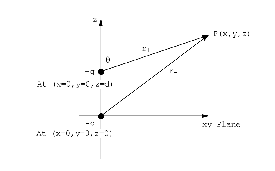
This can be shown as follows (see Figure (2.2.3)):

\[\mathrm{r}_{+}=\left(x^{2}+y^{2}+(z-d)^{2}\right)^{1 / 2}=\left(x^{2}+y^{2}+z^{2}-2 z d+d^{2}\right)^{1 / 2}=\mathrm{r}\left[1-\frac{2 z d}{\mathrm{r}^{2}}+\frac{d^{2}}{\mathrm{r}^{2}}\right]^{1 / 2}. \nonumber \]

Therefore

\[\frac{1}{\mathrm{r}_{+}} \cong \frac{1}{\mathrm{r}}\left[1+\frac{z d}{\mathrm{r}^{2}}\right] \nonumber \]

to first order in the small distance d. Also 1/r₋ = 1/r so that

\[V_{d i p}=\frac{q}{4 \pi \epsilon_{0}} \frac{1}{\mathrm{r}_{+}}-\frac{q}{4 \pi \epsilon_{0}} \frac{1}{\mathrm{r}_{-}} \cong \frac{q z d}{4 \pi \epsilon_{0}} \frac{1}{\mathrm{r}^{3}}. \nonumber\]

But \(\vec p\) = q\(\vec d\) and \(\frac{z}{\mathrm{r}}=\cos (\theta)\) so that V_dip is just given by Equation (\ref{2.14}).

The point dipole potential, Equation (\ref{2.14}), can be used to calculate the potential at the point of observation, \(\vec R\), by superposition of contributions from small volume elements, dV, at \(\vec r\), each of which acts like a point dipole \(\vec p\) = \(\vec P\)dV . The result is

\[ V_{d i p}(\overrightarrow{\mathrm{R}})=\frac{1}{4 \pi \epsilon_{0}} \int_{S p a c e} d V \frac{\overrightarrow{\mathrm{P}} \cdot(\overrightarrow{\mathrm{R}}-\overrightarrow{\mathrm{r}})}{|\overrightarrow{\mathrm{R}}-\overrightarrow{\mathrm{r}}|^{3}}. \label{2.15} \]

Formula (\ref{2.15}) gives the same value for the potential function as does Equation (\ref{2.13}) in which the free charge density, ρ_f , has been set equal to zero. These two ways of calculating the potential due to a distribution of dipoles can be shown to be mathematically equivalent, see Appendix (2A).