1.3: Return to Maxwell’s Equations
- Page ID
- 22715
\( \newcommand{\vecs}[1]{\overset { \scriptstyle \rightharpoonup} {\mathbf{#1}} } \)
\( \newcommand{\vecd}[1]{\overset{-\!-\!\rightharpoonup}{\vphantom{a}\smash {#1}}} \)
\( \newcommand{\id}{\mathrm{id}}\) \( \newcommand{\Span}{\mathrm{span}}\)
( \newcommand{\kernel}{\mathrm{null}\,}\) \( \newcommand{\range}{\mathrm{range}\,}\)
\( \newcommand{\RealPart}{\mathrm{Re}}\) \( \newcommand{\ImaginaryPart}{\mathrm{Im}}\)
\( \newcommand{\Argument}{\mathrm{Arg}}\) \( \newcommand{\norm}[1]{\| #1 \|}\)
\( \newcommand{\inner}[2]{\langle #1, #2 \rangle}\)
\( \newcommand{\Span}{\mathrm{span}}\)
\( \newcommand{\id}{\mathrm{id}}\)
\( \newcommand{\Span}{\mathrm{span}}\)
\( \newcommand{\kernel}{\mathrm{null}\,}\)
\( \newcommand{\range}{\mathrm{range}\,}\)
\( \newcommand{\RealPart}{\mathrm{Re}}\)
\( \newcommand{\ImaginaryPart}{\mathrm{Im}}\)
\( \newcommand{\Argument}{\mathrm{Arg}}\)
\( \newcommand{\norm}[1]{\| #1 \|}\)
\( \newcommand{\inner}[2]{\langle #1, #2 \rangle}\)
\( \newcommand{\Span}{\mathrm{span}}\) \( \newcommand{\AA}{\unicode[.8,0]{x212B}}\)
\( \newcommand{\vectorA}[1]{\vec{#1}} % arrow\)
\( \newcommand{\vectorAt}[1]{\vec{\text{#1}}} % arrow\)
\( \newcommand{\vectorB}[1]{\overset { \scriptstyle \rightharpoonup} {\mathbf{#1}} } \)
\( \newcommand{\vectorC}[1]{\textbf{#1}} \)
\( \newcommand{\vectorD}[1]{\overrightarrow{#1}} \)
\( \newcommand{\vectorDt}[1]{\overrightarrow{\text{#1}}} \)
\( \newcommand{\vectE}[1]{\overset{-\!-\!\rightharpoonup}{\vphantom{a}\smash{\mathbf {#1}}}} \)
\( \newcommand{\vecs}[1]{\overset { \scriptstyle \rightharpoonup} {\mathbf{#1}} } \)
\( \newcommand{\vecd}[1]{\overset{-\!-\!\rightharpoonup}{\vphantom{a}\smash {#1}}} \)
\(\newcommand{\avec}{\mathbf a}\) \(\newcommand{\bvec}{\mathbf b}\) \(\newcommand{\cvec}{\mathbf c}\) \(\newcommand{\dvec}{\mathbf d}\) \(\newcommand{\dtil}{\widetilde{\mathbf d}}\) \(\newcommand{\evec}{\mathbf e}\) \(\newcommand{\fvec}{\mathbf f}\) \(\newcommand{\nvec}{\mathbf n}\) \(\newcommand{\pvec}{\mathbf p}\) \(\newcommand{\qvec}{\mathbf q}\) \(\newcommand{\svec}{\mathbf s}\) \(\newcommand{\tvec}{\mathbf t}\) \(\newcommand{\uvec}{\mathbf u}\) \(\newcommand{\vvec}{\mathbf v}\) \(\newcommand{\wvec}{\mathbf w}\) \(\newcommand{\xvec}{\mathbf x}\) \(\newcommand{\yvec}{\mathbf y}\) \(\newcommand{\zvec}{\mathbf z}\) \(\newcommand{\rvec}{\mathbf r}\) \(\newcommand{\mvec}{\mathbf m}\) \(\newcommand{\zerovec}{\mathbf 0}\) \(\newcommand{\onevec}{\mathbf 1}\) \(\newcommand{\real}{\mathbb R}\) \(\newcommand{\twovec}[2]{\left[\begin{array}{r}#1 \\ #2 \end{array}\right]}\) \(\newcommand{\ctwovec}[2]{\left[\begin{array}{c}#1 \\ #2 \end{array}\right]}\) \(\newcommand{\threevec}[3]{\left[\begin{array}{r}#1 \\ #2 \\ #3 \end{array}\right]}\) \(\newcommand{\cthreevec}[3]{\left[\begin{array}{c}#1 \\ #2 \\ #3 \end{array}\right]}\) \(\newcommand{\fourvec}[4]{\left[\begin{array}{r}#1 \\ #2 \\ #3 \\ #4 \end{array}\right]}\) \(\newcommand{\cfourvec}[4]{\left[\begin{array}{c}#1 \\ #2 \\ #3 \\ #4 \end{array}\right]}\) \(\newcommand{\fivevec}[5]{\left[\begin{array}{r}#1 \\ #2 \\ #3 \\ #4 \\ #5 \\ \end{array}\right]}\) \(\newcommand{\cfivevec}[5]{\left[\begin{array}{c}#1 \\ #2 \\ #3 \\ #4 \\ #5 \\ \end{array}\right]}\) \(\newcommand{\mattwo}[4]{\left[\begin{array}{rr}#1 \amp #2 \\ #3 \amp #4 \\ \end{array}\right]}\) \(\newcommand{\laspan}[1]{\text{Span}\{#1\}}\) \(\newcommand{\bcal}{\cal B}\) \(\newcommand{\ccal}{\cal C}\) \(\newcommand{\scal}{\cal S}\) \(\newcommand{\wcal}{\cal W}\) \(\newcommand{\ecal}{\cal E}\) \(\newcommand{\coords}[2]{\left\{#1\right\}_{#2}}\) \(\newcommand{\gray}[1]{\color{gray}{#1}}\) \(\newcommand{\lgray}[1]{\color{lightgray}{#1}}\) \(\newcommand{\rank}{\operatorname{rank}}\) \(\newcommand{\row}{\text{Row}}\) \(\newcommand{\col}{\text{Col}}\) \(\renewcommand{\row}{\text{Row}}\) \(\newcommand{\nul}{\text{Nul}}\) \(\newcommand{\var}{\text{Var}}\) \(\newcommand{\corr}{\text{corr}}\) \(\newcommand{\len}[1]{\left|#1\right|}\) \(\newcommand{\bbar}{\overline{\bvec}}\) \(\newcommand{\bhat}{\widehat{\bvec}}\) \(\newcommand{\bperp}{\bvec^\perp}\) \(\newcommand{\xhat}{\widehat{\xvec}}\) \(\newcommand{\vhat}{\widehat{\vvec}}\) \(\newcommand{\uhat}{\widehat{\uvec}}\) \(\newcommand{\what}{\widehat{\wvec}}\) \(\newcommand{\Sighat}{\widehat{\Sigma}}\) \(\newcommand{\lt}{<}\) \(\newcommand{\gt}{>}\) \(\newcommand{\amp}{&}\) \(\definecolor{fillinmathshade}{gray}{0.9}\)
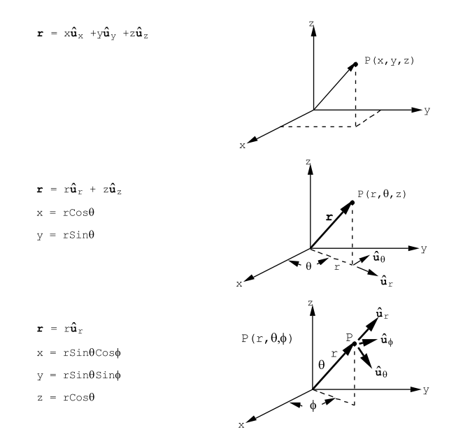
Maxwell’s equations (1.2.1, 1.2.2, 1.2.3, 1.2.4) form a system of differential equations that can be solved for the vector fields \(\vec E\) and \(\vec B\) given the space and time variation of the four source terms ρf(\(\vec r\),t), \(\vec {J_{f}}\)(\(\vec r\),t), \(\vec P\)(\(\vec r\),t), and \(\vec M\)(\(\vec r\),t). In order to solve Maxwell’s equations for a specific problem it is usually convenient to specify each vector field in terms of components in one of the three major co-ordinate systems: (a) cartesian co-ordinates (x,y,z), Figure (1.3.10); (b) cylindrical polar co-ordinates (r,θ,z), Figure (1.3.10); and (c) spherical polar co-ordinates (ρ,θ,φ), Figure (1.3.10).
It is also necessary to be able to calculate the scalar field generated by the divergence of a vector field in each of the above three co-ordinate systems. In addition, one must be able to calculate the three components of the curl in the above three co-ordinate systems. Vector derivatives are reviewed by M.R. Spiegel, Mathematical Handbook of Formulas and Table s, Schaum’s Outline Series, McGraw-Hill, New York, 1968, chapter 22. It is also worthwhile reading the discussion contained in The Feynman Lectures on Physics, by R.P. Feynman, R.B. Leighton, and M. Sands, Addison-Wesley, Reading, Mass., 1964, Volume II, chapters 2 and 3.
The following four vector theorems should be read, understood, and committed to memory because they will be used over and over again in the course of solving Maxwell’s equations.
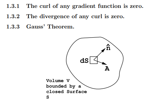
Consider a volume V bounded by a closed surface S, see Figure (1.3.11). An element of area on the surface S can be specified by the vector d\(\vec S\) = \(\hat{n}\)dS where dS is the magnitude of the element of area and \(\hat{n}\) is a unit vector directed along the outward normal to the surface at the element dS. Let \(\vec A\)(\(\vec r\),t) be a vector field that in general may depend upon position and upon time. Then Gauss’ Theorem states that
\[ \int \int_{S}(\vec{\mathrm{A}} \cdot \hat{\mathbf{n}}) d S=\int \int \int_{V} \operatorname{div}(\vec{\mathrm{A}}) d \tau \nonumber\]
where d\(\tau\) is an element of volume. The integrations are to be carried out at a fixed time.
1.3.4 Stokes’ Theorem.
Consider a surface S bounded by a closed curve C, see Figure (1.3.12). \(\vec A\)(\(\vec r\),t) is any vector field that may in general depend upon position and upon time. At
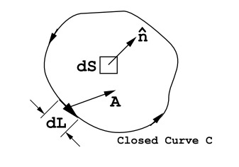
a fixed time calculate the line integral of \(\vec A\) around the curve C; the element of length along the line C is \(d\overrightarrow{\mathrm{L}}\). Then Stokes’ Theorem states that
\[\int_{C} \overrightarrow{\mathrm{A}} \cdot \overrightarrow{d \mathbf{L}}=\iint_{S} \operatorname{curl}(\overrightarrow{\mathrm{A}}) \cdot \hat{\mathbf{n}} d S \nonumber \]
where \(\hat{n}\) is a unit vector normal to the surface element dS whose direction is related to the direction of traversal around the curve C by the right hand rule.