1.3: Gauss’s Law and electrostatic fields and potentials

While the Lorentz force law defines how electric and magnetic fields can be observed, Maxwell’s four equations explain how these fields can be created directly from charges and currents, or indirectly and equivalently from other time varying fields. One of those four equations is Gauss’s Law for charge, which states that the total charge Q [Coulombs] within volume V equals the integral of the normal component of the electric displacement vector \(\vec D\) over the surface area A of that volume:

\[ \oiint _{\text{A}}(\vec{\text{D}} \bullet \hat{n}) \text{d} \text{a}=\int \int \int_{\text{V}} \rho \text{d} \text{v}=\text{Q}\]

In vacuum:

\[\vec{\text{D}}=\varepsilon_{\text{o}} \vec{\text{E}}\]

where the permittivity of vacuum ε_o = 8.854×10^-12 Farads/m. Equation (1.3.1) reveals the dimensions of \(\vec D\): Coulombs/m² , often abbreviated here as [C/m² ].

A few simple examples illustrate typical electric fields for common charge distributions, and how Gauss’s law can be used to compute those fields. First consider a sphere of radius R uniformly filled with charge of density ρ_o [C/m³ ], as illustrated in Figure 1.3.1(a).

Figure 1.3.1: Electric fields \(\vec E\)(r) produced by uniformly charged spheres and cylinders.

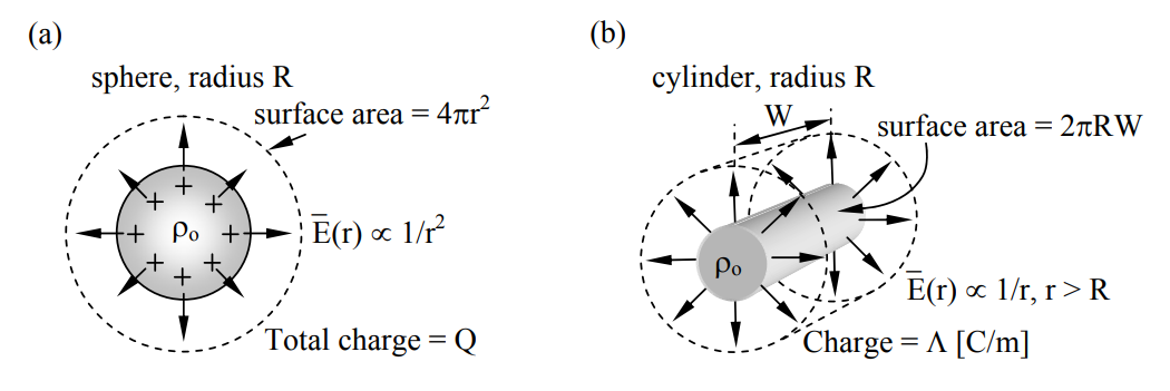
The symmetry of the solution must match the spherical symmetry of the problem, so \(\vec E\) must be independent of θ and \(\Phi\), although it can depend on radius r. This symmetry requires that \(\vec E\) be radial and, more particularly:

\[\vec{\text{E}}(\text{r}, \theta, \phi)=\hat{\text{r}} \text{E}(\text{r})[\text{V} / \text{m}]\]

We can find \(\vec E\)(r) by substituting (1.3.3) into (1.3.1). First consider r > R, for which (1.3.1) becomes:

\[4 \pi r^{2} \varepsilon_{0} E(r)=(4 / 3) \pi R^{3} \rho_{0}=Q\]

\[\vec{\text{E}}(\text{r})=\hat{\text{r}} \frac{\text{Q}}{4 \pi \varepsilon_{0} \text{r}^{2}}\quad \quad \quad (\text{r}>\text{R})\]

Inside the sphere the same substitution into (1.3.1) yields:

\[4 \pi r^{2} \varepsilon_{0} E(r)=(4 / 3) \pi r^{3} \rho_{0}\]

\[\vec{\text{E}}(\text{r})=\hat{\text{r}} \rho_{\text{o}} \text{r} / 3 \varepsilon_{\text{o}}[\text{V} / \text{m}] \quad \quad \quad (\text{r}<\text{R})\]

It is interesting to compare this dependence of \(\vec E\) on r with that for cylindrical geometries, which are also illustrated in Figure 1.3.1. We assume a uniform charge density of ρ_o within radius R, corresponding to Λ coulombs/meter. Substitution of (1.3.4) into (1.3.1) yields:

\[2 \pi r W \varepsilon_{0} E(r)=\pi R^{2} \rho_{o} W=\Lambda W \quad [C] \quad \quad \quad (r>R)\]

\[\vec{\text{E}}(\text{r})=\hat{\text{r}} \frac{\Lambda}{2 \pi \varepsilon_{\text{o}} \text{r}}=\hat{\text{r}} \frac{\text{R}^{2} \rho_{\text{o}}}{2 \varepsilon_{\text{o}} \text{r}}[\text{V} / \text{m}] \quad\quad\quad (\text{r}>\text{R})\]

Inside the cylinder (r < R) the right-hand-side of (1.3.9) still applies, but with R² replaced with r² , so \( \vec{\text{E}}(\text{r})=\hat{\text{r}} \text{r} \rho_{\text{o}} / 2 \varepsilon_{\text{o}}\) instead.

To find the voltage difference, often called the difference in electrical potential \(\Phi\) or the potential difference, between two points in space [V], we can simply integrate the static electric field \(\bar{E} \cdot \hat{r} \) [V/m] along the field line \(\vec E\) connecting them. Thus in the spherical case the voltage difference \(\Phi\left(\text{r}_{1}\right)-\Phi\left(\text{r}_{2}\right) \) between points at r₁ and at r₂ > r₁ is:

\[\Phi\left(\text{r}_{1}\right)-\Phi\left(\text{r}_{2}\right)=\int_{\text{r}_{1}}^{\text{r}_{2}} \vec{\text{E}} \bullet \text{d} \vec{\text{r}}=\frac{\text{Q}}{4 \pi \varepsilon_{\text{o}}} \int_{\text{r}_{1}}^{\text{r}_{2}} \frac{1}{\text{r}^{2}} \hat{\text{r}} \cdot \text{d} \vec{\text{r}}=-\left.\frac{\text{Q}}{4 \pi \varepsilon_{\text{o}} \text{r}}\right|_{\text{r}_{1}} ^{\text{r}_{2}}=\frac{\text{Q}}{4 \pi \varepsilon_{\text{o}}}\left(\frac{1}{\text{r}_{1}}-\frac{1}{\text{r}_{2}}\right)[\text{V}]\]

If we want to assign an absolute value to electrical potential or voltage V at a given location, we usually define the potential \(\Phi\) to be zero at r₂ = ∞, so a spherical charge Q produces an electric potential \(\Phi\)(r) for r > R which is:

\[\Phi(\text{r})=\text{Q} / 4 \pi \varepsilon_{\text{o}} \text{r}[\text{V}]\]

The same computation for the cylindrical charge of Figure 1.3.1 and the field of (1.3.9) yields:

\[\Phi\left(\text{r}_{1}\right)-\Phi\left(\text{r}_{2}\right)=\int_{\text{r}_{1}}^{\text{r}_{2}} \vec{\text{E}} \bullet \text{d} \vec{\text{r}}=\frac{\Lambda}{2 \pi \varepsilon_{\text{o}}} \int_{\text{r}_{1}}^{\text{r}_{2}} \frac{1}{\text{r}} \hat{\text{r}} \cdot \text{d} \vec{\text{r}}=\left.\frac{\Lambda \ln \text{r}}{2 \pi \varepsilon_{\text{o}}}\right|_{\text{r}_{1}} ^{\text{r}_{2}}=\frac{\Lambda}{2 \pi \varepsilon_{\text{o}}} \ln \left(\text{r}_{2} / \text{r}_{1}\right)\]

A third simple geometry is that of charged infinite parallel conducting plates separated by distance d, where the inner-facing surfaces of the upper and lower plates have surface charge density +ρ_s and -ρ_s [C/m² ], respectively, as illustrated in Figure 1.3.2 for finite plates. The uniformity of infinite plates with respect to x, y, and \(\Phi\) requires that the solution \(\vec E\) also be independent of x, y, and \(\Phi\). The symmetry with respect to \(\Phi\) requires that \(\vec E\) point in the ±z direction. Gauss’s law (1.3.1) then requires that \(\vec E\) be independent of z because the integrals of \(\vec D\) over the top and bottom surfaces of any rectangular volume located between the plates must cancel since there is no charge within such a volume and no \(\vec D\) passing through its sides.

Figure 1.3.2: Electric field between parallel plates.

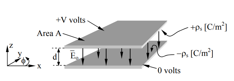
his solution for \(\vec E\) is consistent with the rubber-band model for field lines, which suggests that the excess positive and negative charges will be mutually attracted, and therefore will be pulled to the inner surfaces of the two plates, particularly if the gap d between the plates is small compared to their width. Gauss’s Law (1.3.1) also tells us that the displacement vector \(\vec D\) integrated over a surface enclosing the entire structure must be zero because the integrated charge within that surface is zero; that is, the integrated positive charge, ρ_sA, balances the integrated negative charge, - ρ_sA and \(\vec D\) external to the device can be zero everywhere. The electric potential difference V between the two plates can be found by integrating \(\vec E\) between the two plates. That is, V = E_od volts for any path of integration, where E_o = ρ_s/ε_o by Gauss’s law.

Although the voltage difference between equipotentials can be computed by integrating along the electric field lines themselves, as done above, it is easy to show that the result does not depend on the path of integration. Assume there are two different paths of integration P₁ and P₂ between any two points of interest, and that the two resulting voltage differences are V₁ and V₂. Now consider the closed contour C of integration that is along path P₁ in the positive direction and along P₂ in the reverse direction so as to make a closed loop. Since this contour integral must yield zero, as shown below in (1.3.13) using Faraday’s law for the static case where ∂/∂t = 0, it follows that V₁ = V₂ and that all paths of integration yield the same voltage difference.

\[\text{V}_{1}-\text{V}_{2}=\int_{\text{P}_{1}} \vec{\text{E}} \cdot \text{d} \vec{\text{s}}-\int_{\text{P}_{2}} \vec{\text{E}} \cdot \text{d} \vec{\text{s}}=\oint_{\text{c}} \vec{\text{E}} \cdot \text{d} \vec{\text{s}}=-\frac{\partial}{\partial \text{t}} \int \int_{\text{A}} \vec{\text{B}} \cdot \text{d} \vec{\text{a}}=0\]

In summary, electric fields decay as 1/r² from spherical charge concentrations, as 1/r from cylindrical ones, and are uniform in planar geometries. The corresponding electric potentials decay as 1/r, -ln r, and x, respectively, as a result of integration over distance. The potential \(\Phi\) for the cylindrical case becomes infinite as r→∞ because the cylinder is infinitely long; the expression for the potential difference between concentric cylinders of finite radius is valid, however. Within both uniform spherical and cylindrical charge distributions the electric field increases from zero linearly with radius r. In each case the electric field distribution is explained by the rubber-band model in which the rubber bands (field lines) repel each other laterally while being pulled on by opposite electric charges.

It is extremely useful to note that Maxwell’s equations are linear, so that superposition applies. That is, the total electric field \(\vec E\) equals that due to the sum of all charges present, where the contribution to \(\vec E\) from each charge Q is given by (1.3.5). Electric potentials \(\Phi\) also superimpose, where the contribution from each charge Q is given by (1.3.11).