2.4: Relation between integral and differential forms of Maxwell’s equations

Gauss’s divergence theorem

Two theorems are very useful in relating the differential and integral forms of Maxwell’s equations: Gauss’s divergence theorem and Stokes theorem. Gauss’s divergence theorem (2.1.20) states that the integral of the normal component of an arbitrary analytic overlinetor field \(\overline A \) over a surface S that bounds the volume V equals the volume integral of \( \nabla \cdot \overline{\mathrm{A}}\) over V. The theorem can be derived quickly by recalling (2.1.3):

\[\nabla \cdot \overline{A} \equiv \frac{\partial A_{x}}{\partial x}+\frac{\partial A_{y}}{\partial y}+\frac{\partial A_{z}}{\partial z} \]

Therefore \( \nabla \cdot \overline{A}\) at the position x_o, y_o, z_o can be found using (2.4.1) in the limit where Δx, Δy, and Δz approach zero:

\[\begin{align}
\nabla \cdot \overline{A}=\lim _{\Delta i \rightarrow 0} &\left\{\left[A_{x}\left(x_{0}+\Delta x / 2\right)-A_{x}\left(x_{0}-\Delta x / 2\right)\right] / \Delta x\right.\\
&+\left[A_{y}\left(y_{0}+\Delta y / 2\right)-A_{y}\left(y_{0}-\Delta y / 2\right)\right] / \Delta y \nonumber\\
&\left.+\left[A_{z}\left(z_{0}+\Delta z / 2\right)-A_{z}\left(z_{0}-\Delta z / 2\right)\right] / \Delta z\right\} \nonumber
\end{align} \]

\[\begin{align}
=\lim _{\Delta i \rightarrow 0} &\left\{\Delta y \Delta z\left[A_{x}\left(x_{0}+\Delta x / 2\right)-A_{x}\left(x_{0}-\Delta x / 2\right)\right]\right.\\
&+\Delta x \Delta z\left[A_{y}\left(y_{0}+\Delta y / 2\right)-A_{y}\left(y_{0}-\Delta y / 2\right)\right] \nonumber\\
&\left.+\Delta x \Delta y\left[A_{z}\left(z_{0}+\Delta z / 2\right)-A_{z}\left(z_{0}-\Delta z / 2\right)\right]\right\} / \Delta x \Delta y \Delta z \nonumber
\end{align} \]

\[ =\lim _{\Delta \mathbf{v} \rightarrow 0}\left\{\oiint_{\mathrm{S}_{\mathrm{c}}} \overline{\mathrm{A}} \bullet \hat{n} \mathrm{da} / \Delta \mathrm{v}\right\}\]

where \(\hat{n}\) is the unit normal overlinetor for an incremental cube of dimensions Δx, Δy, Δz; da is its differential surface area; S_c is its surface area; and Δv is its volume, as suggested in Figure 2.4.1(a).

We may now stack an arbitrary number of such infinitesimal cubes to form a volume V such as that shown in Figure 2.4.1(b). Then we can sum (2.4.4) over all these cubes to obtain:

\[ \lim _{\Delta v \rightarrow 0} \sum_{i}(\nabla \bullet \overline{A}) \Delta v_{i}=\lim _{\Delta v \rightarrow 0} \sum_{i}\left\{\oiint_{S_{c}} \overline{A} \bullet \hat{n} d a_{i}\right\}\]

Figure \(\PageIndex{1}\): Derivation of Gauss’s divergence theorem.

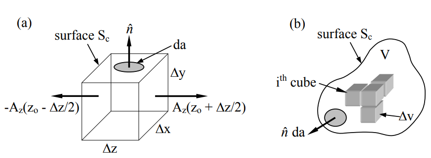
Since all contributions to \(\sum_{i}\left\{\oiint_{S} \overline{A} \bullet \hat{n} d a_{i}\right\} \) from interior-facing adjacent cube faces cancel, the only remaining contributions from the right-hand side of (2.4.5) are from the outer surface of the volume V. Proceeding to the limit, we obtain Gauss’s divergence theorem:

\[ \iiint_{V}(\nabla \bullet \overline{A}) d v=\oiint_{S}(\overline{A} \cdot \hat{n}) d a\]

Stokes’ theorem

Stokes’ theorem states that the integral of the curl of a overlinetor field over a bounded surface equals the line integral of that overlinetor field along the contour C bounding that surface. Its derivation is similar to that for Gauss’s divergence theorem (Section 2.4.1), starting with the definition of the z component of the curl operator [from Equation (2.1.4)]:

\[ (\nabla \times \overline{\mathrm{A}})_{\mathrm{z}} \equiv \hat{z}\left(\frac{\partial \mathrm{A}_{\mathrm{y}}}{\partial \mathrm{x}}-\frac{\partial \mathrm{A}_{\mathrm{x}}}{\partial \mathrm{y}}\right)\]

\[ \begin{align}
=\hat{z} \lim _{\Delta x, \Delta y \rightarrow 0} &\left\{\left[A_{y}\left(x_{0}+\Delta x / 2\right)-A_{y}\left(x_{0}-\Delta x / 2\right)\right] / \Delta x\right.\\
&\left.-\left[A_{x}\left(y_{0}+\Delta y / 2\right)-A_{x}\left(y_{0}-\Delta y / 2\right)\right] / \Delta y\right\}\nonumber
\end{align}\]

\[ \begin{align}
=\hat{z} \lim _{\Delta x, \Delta y \rightarrow 0}\{& \Delta y\left[A_{y}\left(x_{0}+\Delta x / 2\right)-A_{y}\left(x_{0}-\Delta x / 2\right)\right] / \Delta x \Delta y \\
&\left.-\Delta x\left[A_{x}\left(y_{0}+\Delta y / 2\right)-A_{x}\left(y_{0}-\Delta y / 2\right)\right] / \Delta x \Delta y\right\} \nonumber
\end{align}\]

Consider a surface in the x-y plane, perpendicular to \(\hat{z}\) and \(\hat{n}\), the local surface normal, as illustrated in Figure 2.4.2(a).

Figure \(\PageIndex{2}\): Derivation of Stokes’ theorem.

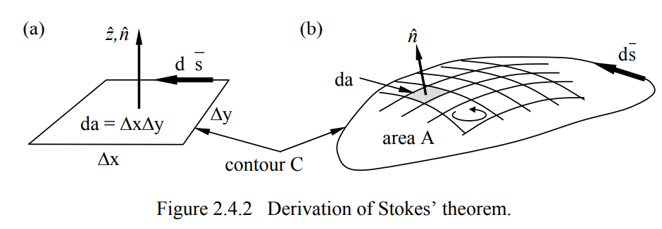
Then (2.4.9) applied to ΔxΔy becomes:

\[\Delta \mathrm{x} \Delta \mathrm{y}(\nabla \times \overline{\mathrm{A}}) \bullet \hat{n}=\oint_{\mathrm{C}} \overline{\mathrm{A}} \bullet \mathrm{d} \overline{\mathrm{s}} \]

where d\(\overline s\) is a overlinetor differential length [m] along the contour C bounding the incremental area defined by ΔxΔy = da. The contour C is transversed in a right-hand sense relative to \(\hat{n}\). We can assemble such infinitesimal areas to form surfaces of arbitrary shapes and area A, as suggested in Figure 2.4.2(b). When we sum (2.4.10) over all these infinitesimal areas da, we find that all contributions to the right-hand side interior to the area A cancel, leaving only the contributions from contour C along the border of A. Thus (2.4.10) becomes Stokes’ theorem:

\[ \int \int_{\mathrm{A}}(\nabla \times \overline{\mathrm{A}}) \bullet \hat{n} \mathrm{da}=\oint_{\mathrm{C}} \overline{\mathrm{A}} \cdot \mathrm{d} \overline{\mathrm{s}}\]

where the relation between the direction of integration around the loop and the orientation of \(\hat{n}\) obey the right-hand rule (if the right-hand fingers curl in the direction of d\(\overline s\), then the thumb points in the direction \(\hat{n}\)).

Maxwell’s equations in integral form

The differential form of Maxwell’s equations (2.1.5–8) can be converted to integral form using Gauss’s divergence theorem and Stokes’ theorem. Faraday’s law (2.1.5) is:

\[\nabla \times \overline{\mathrm{E}}=-\frac{\partial \overline{\mathrm{B}}}{\partial \mathrm{t}} \]

Applying Stokes’ theorem (2.4.11) to the curved surface A bounded by the contour C, we obtain:

\[ \iint_{\mathrm{A}}(\nabla \times \overline{\mathrm{E}}) \bullet \hat{n} \mathrm{d} \mathrm{a}=\oint_{\mathrm{C}} \overline{\mathrm{E}} \bullet \mathrm{d} \overline{\mathrm{s}}=-\iint_{\mathrm{A}} \frac{\partial \overline{\mathrm{B}}}{\partial \mathrm{t}} \bullet \hat{n} \mathrm{d} \mathrm{a}\]

This becomes the integral form of Faraday’s law:

\[\oint_{C} \overline{E} \bullet d \overline{s}=-\frac{\partial}{\partial t} \iint_{A} \overline{B} \bullet \hat{n} d a \quad\quad\quad\quad\quad(\text {Faraday's } L a w)\]

A similar application of Stokes’ theorem to the differential form of Ampere’s law yields its integral form:

\[ \oint_{\mathrm{C}} \overline{\mathrm{H}} \bullet \mathrm{d} \overline{\mathrm{s}}=\iint_{\mathrm{A}}\left[\overline{\mathrm{J}}+\frac{\partial \overline{\mathrm{D}}}{\partial \mathrm{t}}\right] \bullet \hat{n} \mathrm{d} \mathrm{a} \quad\quad\quad\quad\quad \text { (Ampere's Law) }\]

Gauss’s divergence theorem (2.1.20) can be similarly applied to Gauss’s laws to yield their integral form:

\[\int \int \int_{V}(\nabla \bullet \overline{D}) d v=\int \int \int_{V} \rho d v=\oiint_{A}(\overline{D} \bullet \hat{n}) d a \]

This conversion procedure thus yields the integral forms of Gauss’s laws. That is, we can integrate \( \) and \( \) in the differential equations over the surface A that bounds the volume V:

\[ \oiint_{\mathrm{A}}(\overline{\mathrm{D}} \bullet \hat{n}) \mathrm{d} \mathrm{a}=\int \int \int_{\mathrm{V}} \rho \mathrm{d} \mathrm{v} \quad\quad\quad\quad\quad\left(\text {Gauss}^{\prime} s \text { Law for charge}\right)\]

\[\oiint_{\mathrm{A}}(\overline{\mathrm{B}} \bullet \hat{n}) \mathrm{d} \mathrm{a}=0 \quad \quad \quad \quad \quad \text{ (Gauss’s Law for } \overline{B}) \]

Finally, conservation of charge (1.3.19) can be converted to integral form as were Gauss’s laws:

\[ \oiint_{\mathrm{A}}(\overline{\mathrm{J}} \bullet \hat{n}) \mathrm{d} \mathrm{a}=-\int \int \int_{\mathrm{V}} \frac{\partial \rho}{\partial \mathrm{t}} \mathrm{d} \mathrm{v} \quad\quad\quad\quad \quad(\text { conservation of charge })\]

Figure \(\PageIndex{3}\): Maxwell’s equations in sketch form.

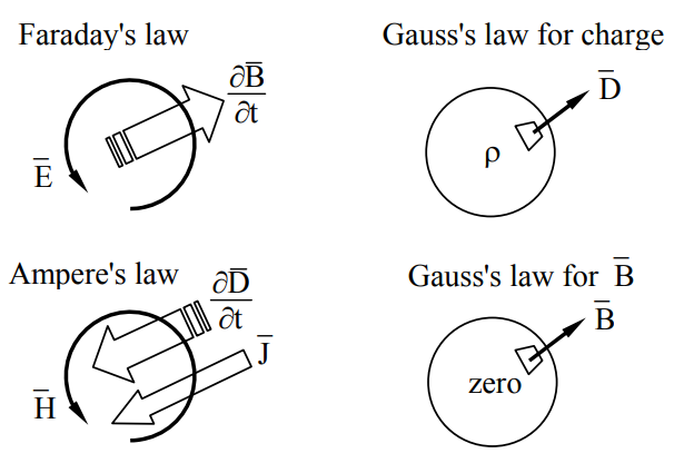
The four sketches of Maxwell’s equations presented in Figure 2.4.3 may facilitate memorization; they can be interpreted in either differential or integral form because they capture the underlying physics.

Example \(\PageIndex{A}\)

Using Gauss’s law, find \(\overline E\) at distance r from a point charge q.

Solution

The spherical symmetry of the problem requires \(\overline E\) to be radial, and Gauss’s law requires \( \int_{\mathrm{A}} \varepsilon_{\mathrm{o}} \overline{\mathrm{E}} \bullet \hat{r} \mathrm{d} \mathrm{A}=\int_{\mathrm{V}} \rho \mathrm{d} \mathrm{v}=\mathrm{q}=4 \pi \mathrm{r}^{2} \varepsilon_{\mathrm{o}} \mathrm{E}_{\mathrm{r}}\), so \(\overline{\mathrm{E}}=\hat{r} \mathrm{E}_{\mathrm{r}}=\hat{r} \mathrm{q} / 4 \pi \varepsilon_{\mathrm{o}} \mathrm{r}^{2}\).

Example \(\PageIndex{B}\)

What is \(\overline H\) at r = 1 cm from a line current \(\overline I\) = \(\hat{z}\) [amperes] positioned at r = 0?

Solution

Because the geometry of this problem is cylindrically symmetric, so is the solution. Using the integral form of Ampere’s law (2.4.15) and integrating in a right-hand sense around a circle of radius r centered on the current and in a plane orthogonal to it, we obtain 2\(\pi\)rH = I, so \(\overline H\) = \(\hat{\theta}\) 100/2\(\pi\) [A m^-1].