5.3: Forces on Bound Charges within Materials

Introduction

Forces on materials can be calculated in three different ways: 1) via the Lorentz force law, as illustrated in Section 5.2 for free charges within materials, 2) via energy methods, as illustrated in Section 5.4, and 3) via photonic forces, as discussed in Section 5.6. When polarized or magnetized materials are present, as discussed here in Section 5.3, the Lorentz force law must be applied not only to the free charges within the materials, i.e. the surface charges and currents discussed earlier, but also to the orbiting and spinning charges bound within atoms. When the Lorenz force equation is applied to these bound charges, the result is the Kelvin polarization and magnetization force densities. Under the paradigm developed in this chapter these Kelvin forces must be added to the Lorentz forces on the free charges¹⁶. The Kelvin force densities are nonzero only when inhomogeneous fields are present, as discussed below in Sections 5.3.2 and 5.3.3. But before discussing Kelvin forces it is useful to review the relationship between the Lorentz force law and matter.

The Lorentz force law is complete and exact if we ignore relativistic issues associated with either extremely high velocities or field strengths; neither circumstance is relevant to current commercial products. To compute all the Lorentz forces on matter we must recognize that classical matter is composed of atoms comprised of positive and negative charges, some of which are moving and exhibit magnetic moments due to their spin or orbital motions. Because these charges are trapped in the matter, any forces on them are transferred to that matter, as assumed in Section 5.2 for electric forces on surface charges and for magnetic forces on surface currents.

When applying the Lorentz force law within matter under our paradigm it is important to use the expression:

\[\overline{\mathrm{f}}=\mathrm{q}\left(\overline{\mathrm{E}}+\overline{\mathrm{v}} \times \mu_{\mathrm{o}} \overline{\mathrm{H}}\right) \quad[\text { Newtons }]\]

without substituting \(\mu \overline{\mathrm{H}}\) for the last term when μ ≠ μ_o. A simple example illustrates the dangers of this common notational shortcut. Consider the instantaneous magnetic pressure (5.2.13) derived using the Lorentz force law for a uniform plane wave normally incident on a conducting plate having μ ≠ μ_o. The same force is also found later in (5.6.5) using photon momentum. If we incorrectly use:

\[\overline{\mathrm{f}}=\mathrm{q}(\overline{\mathrm{E}}+\overline{\mathrm{v}} \times \mu \overline{\mathrm{H}})\ [\text { Newtons }] \qquad\qquad\qquad \text { (incorrect for this example) }\]

¹⁶ The division here between Lorentz forces acting on free charges and the Lorentz forces acting on bound charges (often called Kelvin forces) is complete and accurate, but not unique, for these forces can be grouped and labeled differently, leading to slightly different expressions that are also correct.

because \(\overline{\mathrm{v}}\) occurs within μ, then the computed wave pressure would increase with μ, whereas the photon model has no such dependence and yields \(P_m = μ_oH²/2), the same answer as does (5.2.13). The photon model depends purely on the input and output photon momentum fluxes observed some distance from the mirror, and thus the details of the mirror construction are irrelevant once the fraction of photons reflected is known.

This independence of the Lorentz force from μ can also be seen directly from the Lorentz force calculation that led to (5.2.13). In this case the total surface current is not a function of μ for a perfect reflector, and neither is \(\overline{\mathrm{H}} \) just below the surface; they depend only upon the incident wave and the fact that the mirror is nearly perfect. \( \overline{\mathrm{H}}\) does decay faster with depth when μ is large, as discussed in Section 9.3, but the average |\(\overline{\mathrm{H}}\)| experienced by the surfacecurrent electrons is still half the value of \( \overline{\mathrm{H}}\) at the surface, so \( \overline{\mathrm{f}}\) is unchanged as μ varies. The form of the Lorentz force law presented in (5.3.2) can therefore be safely used under our force paradigm only when μ = μ_o, although the magnetic term is often written as \(\overline{\mathrm{v}} \times \overline{\mathrm{B}}\).

There are alternate correct paradigms that use μ in the Lorentz law rather than μ_o, but they interpret Maxwell’s equations slightly differently. These alternative approaches are not discussed here.

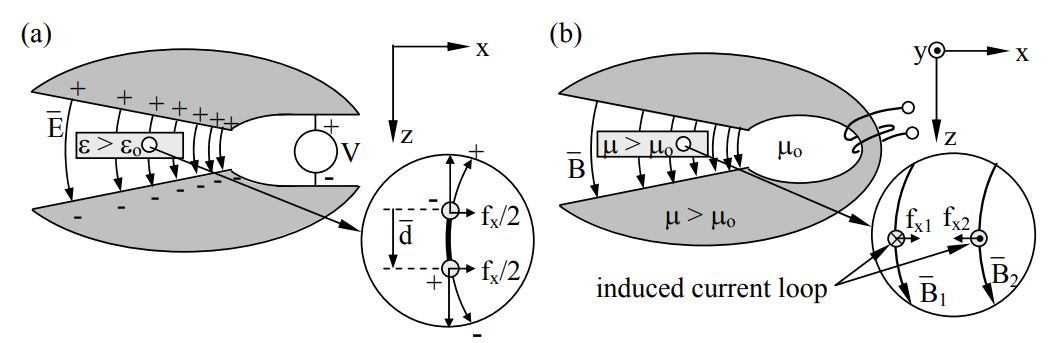
The Lorentz force law can also be applied to those cases where non-uniform fields pull on dielectrics or permeable materials, as suggested by Figure 5.3.1. These problems are often more easily solved, however, using energy (Section 5.4) or pressure (Section 5.5) methods. To compute in general the forces on matter exerted by non-uniform electric or magnetic fields we can derive the Kelvin polarization and magnetization force density expressions from the Lorentz equation, as shown in Sections 5.3.2 and 5.3.3, respectively.

Figure \(\PageIndex{1}\): Kelvin polarization and magnetization forces on materials.

The derivations of the Kelvin force density expressions are based on the following simple models for charges in matter. Electric Lorentz forces act on atomic nuclei and the surrounding electron clouds that are bound together, and on any free charges. The effect of \(\overline{\mathrm{E}}\) on positive and negative charges bound within an atom is to displace their centers slightly, inducing a small electric dipole. The resulting atomic electric dipole moment is:

\[\overline{\mathrm{p}}=\overline{\mathrm{d}} \mathrm{q} \qquad \qquad \qquad \text { (Coulomb meters) }\]

where \(\overline{\mathrm{d}}\) is the displacement vector [m] pointing from the negative charge center to the positive charge center for each atom, and q is the atomic charge or atomic number. As discussed further in Section 5.3.2, Kelvin polarization forces result when the field gradients cause the electric field lines to curve slightly so that the directions of the electric Lorentz forces are slightly different for the two ends of the field-induced electric dipoles so they do not cancel exactly, leaving a net residual force.

The magnetic Lorentz forces act on electrons classically orbiting atomic nuclei with velocities \(\overline{\mathrm{v}}\), and act on electrons with classical charge densities spinning at velocity \(\overline{\mathrm{v}}\) about the electron spin axis. Protons also spin, and therefore both electrons and protons possess magnetic dipole moments; these spin moments are smaller than those due to electron orbital motion. If we consider these spin and orbital motions as being associated with current loops, then we can see that the net force on such a loop would be non-zero if the magnetic fields perpendicular to these currents were different on the two sides of the loop. Such differences exist when the magnetic field has a non-zero gradient and then Kelvin magnetization forces result, as discussed in Section 5.3.3. The electromagnetic properties of matter are discussed further in Sections 2.5 and 9.5.

Kelvin polarization force density

Kelvin polarization forces result when a non-zero electric field gradient causes the Lorentz electric forces on the two charge centers of each induced electric dipole in a dielectric to differ, as illustrated in Figure 5.3.1(a). The force density can be found by summing the force imbalance vectors for each dipole within a unit volume.

Assume the center of the negative charge -q for a particular atom is at \( \overline{\mathrm{r}}\), and the center of the positive charge +q is at \(\overline{\mathrm{r}}+\overline{\mathrm{d}}\). Then the net electric Lorentz force on that atom in the x direction is:

\[f_{x}=q\left[E_{x}(\overline{r}+\overline{d})-E_{x}(\overline{r})\right]=q\left(\overline{d} \bullet \nabla E_{x}\right) \ [N]\]

Thus \(\overline{\mathrm{f}}_{\mathrm{x}} \) is the projection of the charge offset \( \overline{\mathrm{d}}\) on the gradient of qE_x. We recall \(\nabla \equiv \hat{x} \partial / \partial \mathrm{x}+\hat{y} \partial / \partial \mathrm{y}+\hat{z} \partial / \partial \mathrm{z}\).

Equation (5.3.4) can easily be generalized to:

\[\begin{align} \overline{\mathrm{f}} &=\hat{x}\left(\mathrm{q} \overline{\mathrm{d}} \bullet \nabla \mathrm{E}_{\mathrm{x}}\right)+\hat{y}\left(\mathrm{q} \overline{\mathrm{d}} \bullet \nabla \mathrm{E}_{\mathrm{y}}\right)+\hat{z}\left(\mathrm{q} \overline{\mathrm{d}} \bullet \nabla \mathrm{E}_{\mathrm{z}}\right) \\ &=\hat{x}\left(\overline{\mathrm{p}} \bullet \nabla \mathrm{E}_{\mathrm{x}}\right)+\hat{y}\left(\overline{\mathrm{p}} \bullet \nabla \mathrm{E}_{\mathrm{y}}\right)+\hat{z}\left(\overline{\mathrm{p}} \bullet \nabla \mathrm{E}_{\mathrm{z}}\right) \equiv \overline{\mathrm{p}} \bullet \nabla \overline{\mathrm{E}} \quad [\mathrm{N}] \end{align} \]

where \(\overline{\mathrm{p}}=\mathrm{q} \overline{\mathrm{d}}\) and (5.3.6) defines the new compact notation \( \overline{\mathrm{p}} \bullet \nabla \overline{\mathrm{E}}\). Previously we have defined only \(\nabla \times \overline{\mathrm{E}}\) and \(\nabla \bullet \overline{\mathrm{E}}\), and the notation \(\overline{\mathrm{p}} \bullet[.]\) would have implied a scalar, not a vector. Thus the new operator defined here is [•∇], and it operates on a pair of vectors to produce a vector.

Equation (5.3.6) then yields the Kelvin polarization force density \( \overline{\mathrm{F}}_{\mathrm{p}}=\mathrm{n} \overline{\mathrm{f}}\), where n is the density of atomic dipoles [m^-3], and the polarization density of the material \(\overline{\mathrm{P}}\) is \( \mathrm{n} \overline{\mathrm{p}}\) [C m^-2]:

\[\overline{\mathrm{F}}_{\mathrm{p}}=\overline{\mathrm{P}} \bullet \nabla \overline{\mathrm{E}} \quad\left[\mathrm{N} \mathrm{m}^{-3}\right] \qquad\qquad\qquad(\text { Kelvin polarization force density })\]

Equation (5.3.7) states that electrically polarized materials are pulled into regions having stronger electric fields if there is polarization \(\overline{\mathrm{P}} \) in the direction of the gradient. Less obvious from (5.3.7) is the fact that there can be such a force even when the applied electric field \(\overline{\mathrm{E}} \) and \(\overline{\mathrm{P}} \) are orthogonal to the field gradient, as illustrated in Figure 5.3.1(a). In this example a z polarized dielectric is drawn in the x direction into regions of stronger E_z. This happens in curl free fields because then a non-zero ∂E_z/∂x implies a non-zero ∂E_x/∂z that contributes to \(\overline{\mathrm{F}}_{\mathrm{p}}\). This relation between partial derivatives follows from the definition:

\[\nabla \times \overline{\mathrm{E}}=0=\hat{x}\left(\partial \mathrm{E}_{\mathrm{z}} / \partial \mathrm{y}-\partial \mathrm{E}_{\mathrm{y}} / \partial \mathrm{z}\right)+\hat{y}\left(\partial \mathrm{E}_{\mathrm{x}} / \partial \mathrm{z}-\partial \mathrm{E}_{\mathrm{z}} / \partial \mathrm{x}\right)+\hat{z}\left(\partial \mathrm{E}_{\mathrm{y}} / \partial \mathrm{x}-\partial \mathrm{E}_{\mathrm{x}} / \partial \mathrm{y}\right)\]

Since each cartesian component must equal zero, it follows that ∂E_x/∂z = ∂E_z/∂x so both these derivatives are non-zero, as claimed. Note that if the field lines \( \overline{\mathrm{E}}\) were not curved, then f_x = 0 in Figure 5.3.1. But such fields with a gradient ∇E_z ≠ 0 would have non-zero curl, which would require current to flow in the insulating region.

The polarization \(\overline{\mathrm{P}}=\overline{\mathrm{D}}-\varepsilon_{\mathrm{o}} \overline{\mathrm{E}}=\left(\varepsilon-\varepsilon_{\mathrm{o}}\right) \overline{\mathrm{E}} \), as discussed in Section 2.5.3. Thus, in free space, dielectrics with ε > ε_o are always drawn into regions with higher field strengths while dielectrics with ε < ε_o are always repulsed. The same result arises from energy considerations; the total energy we decreases as a dielectric with permittivity ε greater than that of its surrounding ε_o moves into regions having greater field strength \(\overline{\mathrm{E}}\).

Example \(\PageIndex{A}\)

What is the Kelvin polarization force density \( \overline{\mathrm{F}}_{\mathrm{p}}\) [N m^-3] on a dielectric of permittivity ε = 3ε_o in a field \(\overline{\mathrm{E}}=\hat{z} \mathrm{E}_{\mathrm{o}}(1+5 \mathrm{z})\)?

Solution

(5.3.7) yields \(\mathrm{F}_{\mathrm{pz}}=\overline{\mathrm{P}} \bullet\left(\nabla \mathrm{E}_{\mathrm{z}}\right)=\left(\varepsilon-\varepsilon_{\mathrm{o}}\right) \overline{\mathrm{E}} \bullet \hat{z} 5 \mathrm{E}_{\mathrm{o}}=10 \varepsilon_{\mathrm{o}} \mathrm{E}_{\mathrm{o}}^{2}\ \left[\mathrm{N} \mathrm{m}^{-3}\right].\)

Kelvin magnetization force density

Magnetic dipoles are induced in permeable materials by magnetic fields. These induced magnetic dipoles arise when the applied magnetic field slightly realigns the randomly oriented pre-existing magnetic dipoles associated with electron spins and electron orbits in atoms. Each such induced magnetic dipole can be modeled as a small current loop, such as the one pictured in Figure 5.3.1(b) in the x-y plane. The collective effect of these induced atomic magnetic dipoles is a permeability μ that differs from μ_o, as discussed further in Section 2.5.4. Prior to realignment of the magnetic dipoles in a magnetizable medium by an externally applied \(\overline{\mathrm{H}}\), their orientations are generally random so that their effects cancel and can be neglected.

Kelvin magnetization forces on materials result when a non-zero magnetic field gradient causes the Lorentz magnetic forces on the two current centers of each induced magnetic dipole to differ so they no longer cancel, as illustrated in Figure 5.3.1(b). The magnified portion of the figure shows a typical current loop in cross-section where the magnetic Lorentz forces f_x1 and f_x2 are unbalanced because \(\overline{\mathrm{B}}_{1}\) and \( \overline{\mathrm{B}}_{2}\) differ. The magnetic flux density \( \overline{\mathrm{B}}_{1}\) acts on the current flowing in the -y direction, and the magnetic field \(\overline{\mathrm{B}}_{2}\) acts on the equal and opposite current flowing in the +y direction. The force density \( \overline{\mathrm{F}}_{\mathrm{m}}\) can be found by summing the net force vectors for every such induced magnetic dipole within a unit volume. This net force density pulls a medium with μ > μ_o into the high-field region.

The current loops induced in magnetic materials such as iron and nickel tend to increase the applied magnetic field \(\overline{\mathrm{H}} \), as illustrated, so that the permeable material in the figure has μ > μ_o and experiences a net force that tends to move it toward more intense magnetic fields. That is why magnets attract iron and any paramagnetic material that has μ > μ_o, while repulsing any diamagnetic material for which the induced current loops have the opposite polarity so that μ < μ_o. Although most ordinary materials are either paramagnetic or diamagnetic with μ ≅ μ, only ferromagnetic materials such as iron and nickel have μ >> μo and are visibly affected by ordinary magnets.

An expression for the Kelvin magnetization force density \( \overline{\mathrm{F}}_{\mathrm{m}}\) can be derived by calculating the forces on a square current loop of I amperes in the x-y plane, as illustrated. The Lorentz magnetic force on each of the four legs is:

\[\overline{\mathrm{f}}_{\mathrm{i}}=\overline{\mathrm{I}} \times \mu_{\mathrm{o}} \overline{\mathrm{H}} \mathrm{w} \ [\mathrm N]\]

where i = 1,2,3,4, and w is the length of each leg. The sum of these four forces is:

\[\begin{align} \overline{\mathrm{f}} &=\mathrm{Iw}^{2} \mu_{\mathrm{o}}[(\hat{y} \times \partial \overline{\mathrm{H}} / \partial \mathrm{x})-(\hat{x} \times \partial \overline{\mathrm{H}} / \partial \mathrm{y})][\mathrm{N}] \\ &=\mathrm{Iw}^{2} \mu_{\mathrm{o}}\left[-\hat{z}\left(\partial \mathrm{H}_{\mathrm{x}} / \partial \mathrm{x}+\partial \mathrm{H}_{\mathrm{y}} / \partial \mathrm{y}\right)+\hat{x}\left(\partial \mathrm{H}_{\mathrm{z}} / \partial \mathrm{x}\right)+\hat{y}\left(\partial \mathrm{H}_{\mathrm{z}} / \partial \mathrm{y}\right)\right]\nonumber\end{align} \]

This expression can be simplified by noting that \( \overline{\mathrm{m}}=\hat{z} \mathrm{Iw}^{2}\) is the magnetic dipole moment of this current loop, and that \(\partial \mathrm{H}_{\mathrm{x}} / \partial \mathrm{x}+\partial \mathrm{H}_{\mathrm{y}} / \partial \mathrm{y}=-\partial \mathrm{H}_{\mathrm{z}} / \partial \mathrm{z}\) because \(\nabla \bullet \overline{\mathrm{H}}=0 \), while \(\partial \mathrm{H}_{\mathrm{z}} / \partial \mathrm{x}=\partial \mathrm{H}_{\mathrm{x}} / \partial \mathrm{z} \) and \(\partial \mathrm{H}_{\mathrm{z}} / \partial \mathrm{y}=\partial \mathrm{H}_{\mathrm{y}} / \partial \mathrm{z} \) because \(\nabla \times \overline{\mathrm{H}}=0\) in the absence of macroscopic currents. Thus for the geometry of Figure 5.3.1(b), where \( \overline{\mathrm{m}}\) is in the z direction, the magnetization force of Equation (5.3.10) becomes:

\[\overline{\mathrm{f}}_{\mathrm{m}}=\mu_{\mathrm{o}} \mathrm{m}_{\mathrm{z}}\left(\hat{z} \partial \mathrm{H}_{\mathrm{z}} / \partial \mathrm{z}+\hat{x} \partial \mathrm{H}_{\mathrm{x}} / \partial \mathrm{z}+\hat{y} \partial \mathrm{H}_{\mathrm{y}} / \partial \mathrm{z}\right)=\mu_{\mathrm{o}} \mathrm{m}_{\mathrm{z}} \partial \overline{\mathrm{H}} / \partial \mathrm{z}\]

This expression can be generalized to cases where \(\overline{\mathrm{m}}\) is in arbitrary directions:

\[\overline{\mathrm{f}}_{\mathrm{m}}=\mu_{\mathrm{o}}\left(\mathrm{m}_{\mathrm{x}} \partial \overline{\mathrm{H}} / \partial \mathrm{x}+\mathrm{m}_{\mathrm{y}} \partial \overline{\mathrm{H}} / \partial \mathrm{y}+\mathrm{m}_{\mathrm{z}} \partial \overline{\mathrm{H}} / \partial \mathrm{z}\right)=\mu_{\mathrm{o}} \overline{\mathrm{m}} \bullet \nabla \overline{\mathrm{H}} \ [\mathrm N]\]

where the novel notation \(\overline{\mathrm{m}} \bullet \nabla \overline{\mathrm{H}}\) was defined in (5.3.6).

Equation (5.3.12) then yields the Kelvin magnetization force density \(\overline{\mathrm{F}}_{\mathrm{m}}=\mathrm{n}_{3} \overline{\mathrm{f}} \), where n₃ is the equivalent density of magnetic dipoles [m^-3], and the magnetization \(\overline{\mathrm{M}}\) of the material is \(\mathrm{n}_{3} \overline{\mathrm{m}} \) [A m^-1]:

\[\overline{\mathrm{F}}_{\mathrm{m}}=\mu_{\mathrm{o}} \overline{\mathrm{M}} \bullet \nabla \overline{\mathrm{H}}\ \left[\mathrm{N} \mathrm{m}^{-3}\right] \quad(\text { Kelvin magnetization force density })\]

Such forces exist even when the applied magnetic field \(\overline{\mathrm{H}}\) and the magnetization \(v\) are orthogonal to the field gradient, as illustrated in Figure 5.3.1(b). As in the case of Kelvin polarization forces, this happens in curl-free fields because then a non-zero ∂H_z/∂x implies a non-zero ∂H_x/∂z that contributes to \(\overline{\mathrm{F}}_{\mathrm{m}} \).