
6.6: Electric and magnetic sensors


- Last updated
- Jun 7, 2025
- Save as PDF

( \newcommand{\kernel}{\mathrm{null}\,}\)
Electrostatic MEMS sensors
Sensors are devices that respond to their environment. Some sensors alter their properties as a function of the chemical, thermal, radiation, or other properties of the environment, where a separate active circuit probes these properties. The conductivity, permeability, and permittivity of materials are typically sensitive to multiple environmental parameters. Other sensors directly generate voltages in response to the environment that can be amplified and measured. One common MEMS sensor measures small displacements of cantilevered arms due to temperature, pressure, acceleration, chemistry, or other changes. For example, temperature changes can curl a thin cantilever due to differences in thermal expansion coefficient across its thickness, and chemical reactions on the surface of a cantilever can change its mass and mechanical resonance frequency. Microphones can detect vibrations in such cantilevers, or accelerations along specific axes.
Figure 6.6.1 portrays a standard capacitive MEMS sensor that illustrates the basic principles, where the capacitor plates of area A are separated by the distance d, and the voltage V is determined in part by the voltage divider formed by the source resistance Rs and the amplifier input resistance R. Vs is the source voltage.
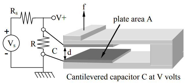
The instantaneous circuit response to an increase δ in the plate separation d is an increase in capacitor voltage V above its normal equilibrium value Ve determined by the voltage divider, where Ve = VsR/(R+Rs). The capacitor then discharges exponentially toward Ve with a time constant τ = (R//Rs)C.29 See Section 3.5.1 Section 3.5.1 for further discussions of RC circuit behavior. If Rs≫R then τ ≅ RC. If Rs≫R and R represents the input resistance of a high-performance sensor amplifier, then that sensor can detect as little as ΔWB≅10−20 joules per “bit of information”30. This can be compared to the incremental increase Δwc in capacitor energy due to the displacement δ≪d as C decreases to C′:
Δwc=(C−C′)V22=V2εoA(d−1−[d+δ]−1)2≅V2εoAδ2d2[J]
A simple example illustrates the extreme potential sensitivity of such a sensor. Assume the plate separation d is one micron, the plates are 1-mm square (A = 10-6), and V = 300. Then the minimum detectable δ given by Equation ??? for Δwc=ΔwB=10−20 Joules is:
δmin
At this potential level of sensitivity we are limited instead by thermal and mechanical noise due to the Brownian motion of air molecules and conduction electrons. A more practical set of parameters might involve a less sensitive detector (ΔB ≅ 10-14) and lower voltages (V ≅ 5); then δmin ≅ 10-10 meters ≅ 1 angstrom (very roughly an atomic diameter). The dynamic range of such a sensor would be enormously greater, of course. This one-angstrom sensitivity is comparable to that of the human eardrum at ~1kHz.
29 The resistance R of two resistors in parallel is \mathrm{R}=\left(\mathrm{R}_{\mathrm{a}} \| \mathrm{R}_{\mathrm{b}}\right)=\mathrm{R}_{\mathrm{a}} \mathrm{R}_{\mathrm{b}} /\left(\mathrm{R}_{\mathrm{a}}+\mathrm{R}_{\mathrm{b}}\right).
30 Most good communications systems can operate with acceptable probabilities of error if Eb/No >~10, where Eb is the energy per bit and No = kT is the noise power density [W Hz-1] = [J]. A bit is a single yes-no piece of information. Boltzmann's constant k ≅ 1.38×10⁻²³ [Jo K-1], and T is the system noise temperature, which might approximate 100K in a good system at RF frequencies. Thus the minimum energy required to detect each bit of information is ~10No = 10 kT ≅ 10-20 [J].
An alternative to such observations of MEMS sensor voltage transients is to observe changes in resonant frequency of an LC resonator that includes the sensor capacitance; this approach can reduce the effects of low-frequency interference.
Magnetic MEMS sensors
Microscopic magnetic sensors are less common than electrostatic ones because of the difficulty of providing strong inexpensive reliable magnetic fields at microscopic scales. High magnetic fields require high currents or strong permanent magnets. If such fields are present, however, mechanical motion of a probe wire or cantilever across the magnetic field lines could produce fluctuating voltages, as given by (6.1.4).
Hall Effect Sensors
Hall effect sensors are semiconductor devices that produce an output voltage VHall proportional to magnetic field \overrightarrow{\mathrm{H}}, where the voltage is produced as a result of magnetic forces on charge carriers moving at velocity \overrightarrow{\mathrm{v}} within the semiconductor. They can measure magnetic fields or, if the magnetic field is known, can determine the average velocity and type (hole or electron) of the charge carriers conveying current. A typical configuration appears in Figure \PageIndex{2}, for which the Hall-effect voltage V_{Hall} is proportional to the current I and to the perpendicular magnetic field \overrightarrow{\mathrm{H}}.
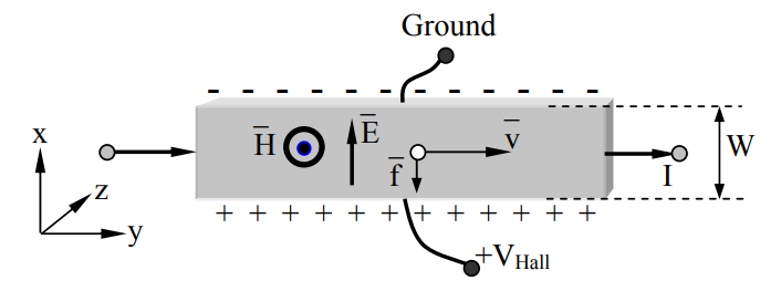
The operation of a Hall-effect sensor follows directly from the Lorentz force law:
\overrightarrow{\mathrm{f}}=\mathrm{q}\left(\overrightarrow{\mathrm{E}}+\overrightarrow{\mathrm{v}} \times \mu_{\mathrm{o}} \overrightarrow{\mathrm{H}}\right)\ [\text { Newtons }] \nonumber
Positively charged carriers moving at velocity \overrightarrow{\mathrm{v}} would be forced downward by \overrightarrow{\mathrm{f}}, as shown in the figure, where they would accumulate until the resulting electric field \overrightarrow{\mathrm{E}} provided a sufficiently strong balancing force qE in the opposite direction to produce equilibrium. In equilibrium the net force and the right-hand side of (6.6.3) must be zero, so \overrightarrow{\mathrm{E}}=-\overrightarrow{\mathrm{v}} \times \mu_{\mathrm{o}} \overrightarrow{\mathrm{H}} and the resulting V_{Hall} is:
\mathrm{V}_{\text {Hall }}=\hat{x} \bullet \overrightarrow{\mathrm{E}} \mathrm{W}=\mathrm{v} \mu_{\mathrm{o}} \mathrm{HW} \ [\mathrm{V}] \nonumber
For charge carrier velocities of 30 m s-1 and fields μoH of 0.1 Tesla, VHall would be 3 millivolts across a width W of one millimeter, which is easily detected.
If the charge carriers are electrons so q < 0, then the sign of the Hall voltage is reversed. Since the voltage depends on the velocity v of the carriers rather than on their number, their average number density N [m-1] can be determined using I = Nqv. That is, for positive carriers:
\mathrm{v}=\mathrm{V}_{\mathrm{H}} / \mathrm{W} \mu_{\mathrm{o}} \mathrm{H} \ \left[\mathrm{ms}^{-1}\right] \nonumber
\mathrm{N}=\mathrm{I} / \mathrm{qv} \nonumber
Thus the Hall effect is useful for understanding carrier behavior (N,v) as a function of semiconductor composition.