Physics LibreTexts

4.15: Solutions, Answers or Hints to 4.14

  • Page ID
    5981
  • \( \newcommand{\vecs}[1]{\overset { \scriptstyle \rightharpoonup} {\mathbf{#1}} } \)

    \( \newcommand{\vecd}[1]{\overset{-\!-\!\rightharpoonup}{\vphantom{a}\smash {#1}}} \)

    \( \newcommand{\id}{\mathrm{id}}\) \( \newcommand{\Span}{\mathrm{span}}\)

    ( \newcommand{\kernel}{\mathrm{null}\,}\) \( \newcommand{\range}{\mathrm{range}\,}\)

    \( \newcommand{\RealPart}{\mathrm{Re}}\) \( \newcommand{\ImaginaryPart}{\mathrm{Im}}\)

    \( \newcommand{\Argument}{\mathrm{Arg}}\) \( \newcommand{\norm}[1]{\| #1 \|}\)

    \( \newcommand{\inner}[2]{\langle #1, #2 \rangle}\)

    \( \newcommand{\Span}{\mathrm{span}}\)

    \( \newcommand{\id}{\mathrm{id}}\)

    \( \newcommand{\Span}{\mathrm{span}}\)

    \( \newcommand{\kernel}{\mathrm{null}\,}\)

    \( \newcommand{\range}{\mathrm{range}\,}\)

    \( \newcommand{\RealPart}{\mathrm{Re}}\)

    \( \newcommand{\ImaginaryPart}{\mathrm{Im}}\)

    \( \newcommand{\Argument}{\mathrm{Arg}}\)

    \( \newcommand{\norm}[1]{\| #1 \|}\)

    \( \newcommand{\inner}[2]{\langle #1, #2 \rangle}\)

    \( \newcommand{\Span}{\mathrm{span}}\) \( \newcommand{\AA}{\unicode[.8,0]{x212B}}\)

    \( \newcommand{\vectorA}[1]{\vec{#1}}      % arrow\)

    \( \newcommand{\vectorAt}[1]{\vec{\text{#1}}}      % arrow\)

    \( \newcommand{\vectorB}[1]{\overset { \scriptstyle \rightharpoonup} {\mathbf{#1}} } \)

    \( \newcommand{\vectorC}[1]{\textbf{#1}} \)

    \( \newcommand{\vectorD}[1]{\overrightarrow{#1}} \)

    \( \newcommand{\vectorDt}[1]{\overrightarrow{\text{#1}}} \)

    \( \newcommand{\vectE}[1]{\overset{-\!-\!\rightharpoonup}{\vphantom{a}\smash{\mathbf {#1}}}} \)

    \( \newcommand{\vecs}[1]{\overset { \scriptstyle \rightharpoonup} {\mathbf{#1}} } \)

    \( \newcommand{\vecd}[1]{\overset{-\!-\!\rightharpoonup}{\vphantom{a}\smash {#1}}} \)

    \(\newcommand{\avec}{\mathbf a}\) \(\newcommand{\bvec}{\mathbf b}\) \(\newcommand{\cvec}{\mathbf c}\) \(\newcommand{\dvec}{\mathbf d}\) \(\newcommand{\dtil}{\widetilde{\mathbf d}}\) \(\newcommand{\evec}{\mathbf e}\) \(\newcommand{\fvec}{\mathbf f}\) \(\newcommand{\nvec}{\mathbf n}\) \(\newcommand{\pvec}{\mathbf p}\) \(\newcommand{\qvec}{\mathbf q}\) \(\newcommand{\svec}{\mathbf s}\) \(\newcommand{\tvec}{\mathbf t}\) \(\newcommand{\uvec}{\mathbf u}\) \(\newcommand{\vvec}{\mathbf v}\) \(\newcommand{\wvec}{\mathbf w}\) \(\newcommand{\xvec}{\mathbf x}\) \(\newcommand{\yvec}{\mathbf y}\) \(\newcommand{\zvec}{\mathbf z}\) \(\newcommand{\rvec}{\mathbf r}\) \(\newcommand{\mvec}{\mathbf m}\) \(\newcommand{\zerovec}{\mathbf 0}\) \(\newcommand{\onevec}{\mathbf 1}\) \(\newcommand{\real}{\mathbb R}\) \(\newcommand{\twovec}[2]{\left[\begin{array}{r}#1 \\ #2 \end{array}\right]}\) \(\newcommand{\ctwovec}[2]{\left[\begin{array}{c}#1 \\ #2 \end{array}\right]}\) \(\newcommand{\threevec}[3]{\left[\begin{array}{r}#1 \\ #2 \\ #3 \end{array}\right]}\) \(\newcommand{\cthreevec}[3]{\left[\begin{array}{c}#1 \\ #2 \\ #3 \end{array}\right]}\) \(\newcommand{\fourvec}[4]{\left[\begin{array}{r}#1 \\ #2 \\ #3 \\ #4 \end{array}\right]}\) \(\newcommand{\cfourvec}[4]{\left[\begin{array}{c}#1 \\ #2 \\ #3 \\ #4 \end{array}\right]}\) \(\newcommand{\fivevec}[5]{\left[\begin{array}{r}#1 \\ #2 \\ #3 \\ #4 \\ #5 \\ \end{array}\right]}\) \(\newcommand{\cfivevec}[5]{\left[\begin{array}{c}#1 \\ #2 \\ #3 \\ #4 \\ #5 \\ \end{array}\right]}\) \(\newcommand{\mattwo}[4]{\left[\begin{array}{rr}#1 \amp #2 \\ #3 \amp #4 \\ \end{array}\right]}\) \(\newcommand{\laspan}[1]{\text{Span}\{#1\}}\) \(\newcommand{\bcal}{\cal B}\) \(\newcommand{\ccal}{\cal C}\) \(\newcommand{\scal}{\cal S}\) \(\newcommand{\wcal}{\cal W}\) \(\newcommand{\ecal}{\cal E}\) \(\newcommand{\coords}[2]{\left\{#1\right\}_{#2}}\) \(\newcommand{\gray}[1]{\color{gray}{#1}}\) \(\newcommand{\lgray}[1]{\color{lightgray}{#1}}\) \(\newcommand{\rank}{\operatorname{rank}}\) \(\newcommand{\row}{\text{Row}}\) \(\newcommand{\col}{\text{Col}}\) \(\renewcommand{\row}{\text{Row}}\) \(\newcommand{\nul}{\text{Nul}}\) \(\newcommand{\var}{\text{Var}}\) \(\newcommand{\corr}{\text{corr}}\) \(\newcommand{\len}[1]{\left|#1\right|}\) \(\newcommand{\bbar}{\overline{\bvec}}\) \(\newcommand{\bhat}{\widehat{\bvec}}\) \(\newcommand{\bperp}{\bvec^\perp}\) \(\newcommand{\xhat}{\widehat{\xvec}}\) \(\newcommand{\vhat}{\widehat{\vvec}}\) \(\newcommand{\uhat}{\widehat{\uvec}}\) \(\newcommand{\what}{\widehat{\wvec}}\) \(\newcommand{\Sighat}{\widehat{\Sigma}}\) \(\newcommand{\lt}{<}\) \(\newcommand{\gt}{>}\) \(\newcommand{\amp}{&}\) \(\definecolor{fillinmathshade}{gray}{0.9}\)

    Hints for 4.14.1. Imagine a current of 6\(I\) going into the bottom left hand corner. Follow the current through the cube, writing down the current through each of the 12 resistors. Also write down the potential drop across each resistor, and hence the total potential drop across the cube. I make the answer for the effective resistance of the whole cube \(\frac{5}{6}r\).

    Solution for 4.14.2. By symmetry, the potentials of A and B are equal. Therefore there is no current between A and B.

    Hint for 4.14.3. Replace the heavily-drawn delta with its corresponding star. After that it should be straightforward, although there is a little bit of calculation to do. I make the answer 1.52 \(\Omega\) .

    Solution for 4.14. From equation 4.8.1, the rate at which heat is generated in a resistance R connected across a battery of EMF E and internal resistance r is \(\frac{E^2R}{(R+r)^2}\). If the resistors are connected in series, \(R=R_1+R_2\) while if they are connected in parallel, \(R+\frac{R_1R_2}{R_1+R_2}\). If the heat generated is the same in either case, we must have

    \[\frac{R_1+R_2}{(R_1+R_2+r)^2}=\frac{\frac{R_1R_2}{R_1+R_2}}{\left ( \frac{R_1R_2}{R_1+R_2}+r \right )^2}.\nonumber\]

    After some algebra, we obtain

    \[r=\frac{R_1+R_2-\sqrt{R_1R_2}}{\sqrt{\frac{R_1}{R_2}}+\sqrt{\frac{R_2}{R_1}}-1}.\label{4.15.1}\]

    With R1 = 8 \(\Omega\) and R2 = 0.5 \(\Omega\), we obtain r = 2.00 \(\Omega\) .

    Solution for 4.14.5.

    In equation 4.15.1, let \(\frac{r}{R_1}\) and \(\sqrt{\frac{R_2}{R_1}}=x\). The equation 4.15.1 becomes

    \[a=\frac{1+x^2-x}{(1/x)+x-1}.\label{4.15.2}\]

    Upon rearrangement, this is

    \[a-(a+1)x+(a+1)x^2-x^3=0 \label{4.15.3}\]

    In our example, \(a=\frac{r}{R_1}=\frac{0.50}{0.25}=2\) so that equation 4.15.4 is

    \[2-3x+3x^2-x^3=0,\nonumber\]

    or

    \[(2-x)(1-x+x^2)=0\nonumber\]

    The only real root is x = 2. But \(R_2=R_1x^2=0.25x^2=1\Omega\).

    Solution to 4.14.6 Suppose that there are n links (2n resistors) to the right of the dotted line, and that the effective resistance of these n links is Rn. Add one more link, to the left. The effective resistance of the n + 1 links is then

    \[R_{n+1}=\frac{2R_n+1}{R_n+1}.\label{4.15.4}\]

    As \(n\to \infty,\,R_{n+1}\to R_n\to R. \therefore R \frac{2R+1}{R+1},\, \text{or }R^2-R-1=0\).

    Whence, \(R=\frac{1}{2}(\sqrt{5}+1)=1.618033989 \Omega \).

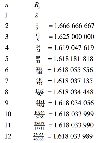
    Solution to 4.14.7 By repeated application of equation 4.15.4, we find:

    4.15 list.png

    Inspection shows that \(R_n=\frac{F_{2n+1}}{F_{2n}},\) where \(F_m\) is the mth member of the Fibonacci sequence: 1 1 2 3 5 8 13 21 ...

    But, from the theory of Fibonacci sequences,

    \[F_m = \frac{1}{\sqrt{5}} \left \{ \left ( \frac{1+\sqrt{5}}{2}\right )^m-\left (\frac{1-\sqrt{5}}{2}\right )^m \right \}.\nonumber\]

    Hence

    \[R_n=\frac{1}{2}\left ( \frac{(1+\sqrt{5})^{2n+1}-(1-\sqrt{5})^{2n+1}}{(1+\sqrt{5})^{2n}-(1-\sqrt{5})^{2n}}\right )\Omega \nonumber \]
    4.14.8 Solutions.png

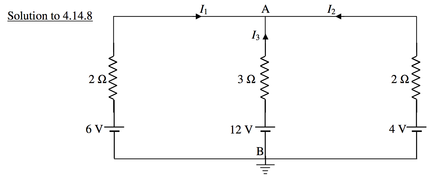
    I’ll call the potential at B (and at the negative poles of each cell) zero, which is equivalent to grounding (earthing) the point B; and I’ll call the potential at A V.

    I don’t think all of the currents will be in the direction indicated on the drawing. One or more must be in the other direction, and one or more of the cells are being re-charged. I don’t know which is wrong, so I’ll just leave them as drawn for the time being, and we’ll see what happens. Apply Ohm’s law to each resistor in turn:

    \(I_1=\frac{V-6}{2};\,I_x=\frac{V-12}{3};\,I_3=\frac{V-4}{2}\) amps, and apply Kirchhoff’s first rule to A: \(I_1+I_2+I_3=0\). From these, we obtain V = 6.750 V, \(I\)1 = 0.375 A, \(I\)2 = -1.75 A, \(I\)2 = 1.375 A.


    This page titled 4.15: Solutions, Answers or Hints to 4.14 is shared under a CC BY-NC 4.0 license and was authored, remixed, and/or curated by Jeremy Tatum via source content that was edited to the style and standards of the LibreTexts platform.

    • Was this article helpful?