4.16: Attenuators

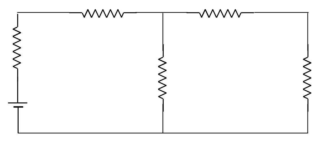
These are networks, usually of resistors, that serve the dual purpose of supplying more examples for students or for reducing the voltage, current or power from one circuit to another. An example of the former might be:

You might be told the values of the four left-hand resistances and of the EMF of the cell, and you are asked to find the current in the right hand resistor.

On the other hand, if the object is to design an attenuator, you might be told the values of the resistances at the two ends, and you are required to find the resistances of the three middle resistors such that the current in the rightmost resistor is half the current in the left hand resistor. The three intermediate resistances perform the function of an attenuator.

In the drawing below, A is some sort of a device, or electrical circuit, or, in the simplest case, just a battery, which has an electromotive force E and an internal resistance R_A. C is some other device, whose internal resistance is R_C. B is an attenuator, which is a collection of resistors which you want to design so that the current delivered to C is a certain fraction of the current flowing from A; or so that the voltage delivered across the terminals of C is a certain fraction of the voltage across the terminals of A; or perhaps again so that the power delivered to C is a certain fraction of the power generated by A. The circuit in the attenuator has to be designed so as to achieve one of these goals.

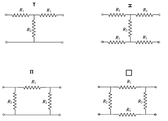
Four simple attenuators are known as T, H, \(\Pi\) or square, named after their shapes. In the drawing below, the H is on its side, like this:

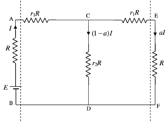
Let us look at a T attenuator. We’ll suppose that the A device has an electromotive force E and an internal resistance R, and indeed it can be represented by a cell in series with a resistor. And we’ll suppose that the resistance of the C device is also R and it can be represented by a single resistor. We’ll suppose that we want the current that flows into C to be a fraction a of the current flowing out of A, and the voltage to be supplied to C to be a fraction a of the potential difference across the output terminals of A. What must be the values of the resistances in the T attenuator? I’ll call them r₁R and r₂R, so that we have to determine the dimensionless ratios r₁ and r₂. The equivalent circuit is:

The current leaving the battery is \(I\), and we want the current entering the load at the right hand side to be a\(I\). The current down the middle resistor is then necessarily, by Kirchhoff’s first rule, \((1-a)I\). If we apply Kirchhoff’s second rule to the outermost circuit, we obtain (after algebraic reduction)

\[E=(1+a)(1+r_1)IR\label{4.16.1}\]

We also want the potential difference across the load (i.e. across EF), which, by Ohm’s law, is a\(I\)R, to be a times the potential difference across the source AB. AB are the terminals of the source. Recall that E is the EMF of the source, and R its internal resistance, so that, when a current I is being taken from the source, the potential difference across its terminals AB is E - \(I\)R, and we want a\(I\)R to be a times this. The fraction a can be called the voltage reduction factor of the attenuator. Thus we have

\[aIR = a(E-IR).\label{4.16.2}\]

From these two equations we obtain

\[r_1 =\frac{1-a}{1+a}\label{4.16.3}\]

Application of Kirchhoff’s second rule to the right hand circuit gives

\[r_2(1-a)IR=a(1+r_1)IR,\label{4.16.4}\]

which, in combination with equation 4.16.3, yields

\[r_2=\frac{2a}{1-a^2}.\label{4.16.5}\]

Thus, if source and load resistance are each equal to R, and we want a voltage reduction factor of \(\frac{1}{2}\), we must choose r₁R to be \(\frac{1}{3}R\), and r₂R to be \(\frac{4}{3}R\).

For :

\[r_1=\frac{1}{2}\left ( \frac{1-a}{1+a}\right ) \quad \quad r_2=\frac{2a}{1-a^2} \label{4.16.6}\]

For \(\Pi\):

\[r_1=\frac{1-a^2}{2a} \quad \quad r_2=\frac{1+a}{1-a}\label{4.16.7}\]

For square:

\[r_1=\frac{1}{2}\left ( \frac{1-a^2}{2a}\right ) \quad \quad r_2=\frac{1+a}{1-a}\label{4.16.8}\]