10.12: Equivalent Circuit Model for Reception, Redux

Section 10.9 provides an informal derivation of an equivalent circuit model for a receiving antenna. This model is shown in Figure $\PageIndex{1}$.

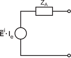Figure $\PageIndex{1}$: Thévenin equivalent circuit model for an antenna in the presence of an incident electric field $\mathbf{E}^{i}$. (CC BY-SA 4.0; S. Lally)

The derivation of this model was informal and incomplete because the open-circuit potential ${\bf E}^i\cdot{\bf l}_e$ and source impedance $Z_A$ were not rigorously derived in that section. While the open-circuit potential was derived in Section 10.11 (“Potential Induced in a Dipole”), the source impedance has not yet been addressed. In this section, the source impedance is derived, which completes the formal derivation of the model. Before reading this section, a review of Section 10.10 (“Reciprocity”) is recommended.

The starting point for a formal derivation is the two-port model shown in Figure $\PageIndex{2}$.

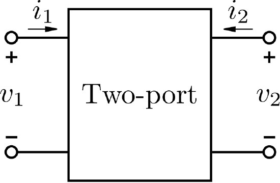Figure $\PageIndex{2}$: Two-port system. (public domain (modified); Inductiveload)

If the two-port is passive, linear, and time-invariant, then the potential $v_2$ is a linear function of potentials and currents present at ports 1 and 2. Furthermore, $v_1$ must be proportional to $i_1$, and similarly $v_2$ must be proportional to $i_2$, so any pair of “inputs” consisting of either potentials or currents completely determines the two remaining potentials or currents. Thus, we may write:

$$v_2 = Z_{21} i_1 + Z_{22} i_2 \label{m0216_ev2}$$

where $Z_{11}$ and $Z_{12}$ are, for the moment, simply constants of proportionality. However, note that $Z_{11}$ and $Z_{12}$ have SI base units of $\Omega$, and so we refer to these quantities as impedances. Similarly we may write:

$$v_1 = Z_{11} i_1 + Z_{12} i_2 \label{m0216_ev1}$$

We can develop expressions for $Z_{12}$ and $Z_{21}$ as follows. First, note that $v_{1}=Z_{12}i_2$ when $i_1=0$. Therefore, we may define $Z_{12}$ as follows:

$$Z_{12} \triangleq \left.\frac{v_1}{i_2}\right|_{i_1=0} \nonumber$$

The simplest way to make $i_1=0$ (leaving $i_2$ as the sole “input”) is to leave port 1 open-circuited. In previous sections, we invoked special notation for these circumstances. In particular, we defined $\widetilde{I}_2^t$ as $i_2$ in phasor representation, with the superscript “$t$” (“transmitter”) indicating that this is the sole “input”; and $\widetilde{V}_1^r$ as $v_1$ in phasor representation, with the superscript “$r$” (“receiver”) signaling that port 1 is both open-circuited and the “output.” Applying this notation, we note:

$$Z_{12} = \frac{\widetilde{V}_1^r}{\widetilde{I}_2^t} \label{m0216_eZ12}$$

Similarly:

$$Z_{21} = \frac{\widetilde{V}_2^r}{\widetilde{I}_1^t} \label{m0216_eZ21}$$

In Section 10.10 (“Reciprocity”), we established that a pair of antennas could be represented as a passive linear time-invariant two-port, with $v_1$ and $i_1$ representing the potential and current at the terminals of one antenna (“antenna 1”), and $v_2$ and $i_2$ representing the potential and current at the terminals of another antenna (“antenna 2”). Therefore for any pair of antennas, quantities $Z_{11}$, $Z_{12}$, $Z_{22}$, and $Z_{21}$ can be identified that completely determine the relationship between the port potentials and currents.

We also established in Section 10.10 that:

$$\widetilde{I}_1^t \widetilde{V}_1^r = \widetilde{I}_2^t \widetilde{V}_2^r \label{m0216_eRIV}$$

Therefore,

$$\frac{\widetilde{V}_1^r}{\widetilde{I}_2^t} = \frac{\widetilde{V}_2^r}{\widetilde{I}_1^t} \label{m0216_eR1}$$

Referring to Equations $\ref{m0216_eZ12}$ and $\ref{m0216_eZ21}$, we see that Equation $\ref{m0216_eR1}$ requires that:

$$Z_{12} = Z_{21} \nonumber$$

This is a key point. Even though we derived this equality by open-circuiting ports one at a time, the equality must hold generally since Equations $\ref{m0216_ev2}$ and $\ref{m0216_ev1}$ must apply – with the same values of $Z_{12}$ and $Z_{21}$ – regardless of the particular values of the port potentials and currents.

We are now ready to determine the Thévenin equivalent circuit for a receiving antenna. Let port 1 correspond to the transmitting antenna; that is, $i_1$ is $\widetilde{I}_1^t$. Let port 2 correspond to an open-circuited receiving antenna; thus, $i_2=0$ and $v_2$ is $\widetilde{V}_2^r$. Now applying Equation $\ref{m0216_ev2}$:

$$\begin{aligned} v_2 &= Z_{21} i_1 + Z_{22} i_2 \nonumber \\ &= \left(\widetilde{V}_2^r/\widetilde{I}_1^t\right) \widetilde{I}_1^t + Z_{22} \cdot 0 \nonumber \\ &= \widetilde{V}_2^r\end{aligned} \nonumber$$

We previously determined $\widetilde{V}_2^r$ from electromagnetic considerations to be (Section 10.11):

$$\widetilde{V}_2^r = \widetilde{\bf E}^i\cdot{\bf l}_e \nonumber$$

where $\widetilde{\bf E}^i$ is the field incident on the receiving antenna, and ${\bf l}_e$ is the vector effective length as defined in Section 10.11. Thus, the voltage source in the Thévenin equivalent circuit for the receive antenna is simply $\widetilde{\bf E}^i\cdot{\bf l}_e$, as shown in Figure $\PageIndex{1}$.

The other component in the Thévenin equivalent circuit is the series impedance. From basic circuit theory, this impedance is the ratio of $v_2$ when port 2 is open-circuited (i.e., $\widetilde{V}_2^r$) to $i_2$ when port 2 is short-circuited. This value of $i_2$ can be obtained using Equation $\ref{m0216_ev2}$ with $v_2=0$:

$$0 = Z_{21} \widetilde{I}_1^t + Z_{22} i_2 \nonumber$$

Therefore:

$$i_2 = - \frac{Z_{21}}{Z_{22}} \widetilde{I}_1^t \nonumber$$

Now using Equation $\ref{m0216_eZ21}$ to eliminate $\widetilde{I}_1^t$, we obtain:

$$i_2 = - \frac{\widetilde{V}_2^r}{Z_{22}} \nonumber$$

Note that the reference direction for $i_2$ as defined in Figure $\PageIndex{2}$ is opposite the reference direction for short-circuit current. That is, given the polarity of $v_2$ shown in Figure $\PageIndex{2}$, the reference direction of current flow through a passive load attached to this port is from “$+$” to “$-$” through the load. Therefore, the source impedance, calculated as the ratio of the open-circuit potential to the short circuit current, is:

$$\frac{\widetilde{V}_2^r}{+\widetilde{V}_2^r/Z_{22}} = Z_{22} \nonumber$$

We have found that the series impedance $Z_A$ in the Thévenin equivalent circuit is equal to $Z_{22}$ in the two-port model.

To determine $Z_{22}$, let us apply a current $i_2=\widetilde{I}_2^t$ to port 2 (i.e., antenna 2). Equation $\ref{m0216_ev2}$ indicates that we should see:

$$v_2 = Z_{21} i_1 + Z_{22} \widetilde{I}_2^t \nonumber$$

Solving for $Z_{22}$:

$$Z_{22} = \frac{v_2}{\widetilde{I}_2^t} - Z_{21} \frac{i_1}{\widetilde{I}_2^t} \label{m0216_eZ22exact}$$

Note that the first term on the right is precisely the impedance of antenna 2 in transmission. The second term in Equation $\ref{m0216_eZ22exact}$ describes a contribution to $Z_{22}$ from antenna 1. However, our immediate interest is in the equivalent circuit for reception of an electric field $\widetilde{\bf E}^i$ in the absence of any other antenna. We can have it both ways by imagining that $\widetilde{\bf E}^i$ is generated by antenna 1, but also that antenna 1 is far enough away to make $Z_{21}$ – the factor that determines the effect of antenna 1 on antenna 2 – negligible. Then we see from Equation $\ref{m0216_eZ22exact}$ that $Z_{22}$ is the impedance of antenna 2 when transmitting.

Summarizing:

The Thévenin equivalent circuit for an antenna in the presence of an incident electric field $\widetilde{\bf E}^i$ is shown in Figure $\PageIndex{1}$. The series impedance $Z_A$ in this model is equal to the impedance of the antenna in transmission.

Mutual coupling

This concludes the derivation, but raises a follow-up question: What if antenna 2 is present and not sufficiently far away that $Z_{21}$ can be assumed to be negligible? In this case, we refer to antenna 1 and antenna 2 as being “coupled,” and refer to the effect of the presence of antenna 1 on antenna 2 as coupling. Often, this issue is referred to as mutual coupling, since the coupling affects both antennas in a reciprocal fashion. It is rare for coupling to be significant between antennas on opposite ends of a radio link. This is apparent from common experience. For example, changes to a receive antenna are not normally seen to affect the electric field incident at other locations. However, coupling becomes important when the antenna system is a dense array; i.e., multiple antennas separated by distances less than a few wavelengths. It is common for coupling among the antennas in a dense array to be significant. Such arrays can be analyzed using a generalized version of the theory presented in this section.