
6.3: Quasistatic Approximation, and the Skin Effect


- Last updated
- Mar 5, 2022
- Save as PDF

( \newcommand{\kernel}{\mathrm{null}\,}\)
Perhaps the most surprising experimental fact concerning the time-dependent electromagnetic phenomena is that unless they are so fast that one more new effect of the displacement currents (to be discussed in Sec. 7 below) becomes noticeable, all formulas of electrostatics and magnetostatics remain valid, with the only exception: the generalization of Eq. (3.36) to Eq. (5), describing the Faraday induction. As a result, the system of macroscopic Maxwell equations (5.109) is generalized to
∇×E+∂B∂t=0,∇×H=j,∇⋅D=ρ,∇⋅B=0.Quasistatic approximation
(As it follows from the discussions in chapters 3 and 5, the corresponding system of microscopic Maxwell equations for the genuine, “microscopic” fields E and B may be obtained from Eq. (21) by the formal substitutions D=ε0E and H=B/μ0, and the replacement of the stand-alone charge and current densities ρ and j with their full densities.11) These equations, whose range of validity will be quantified in Sec. 7, define the so-called quasistatic approximation of electromagnetism and are sufficient for an adequate description of a broad range of physical effects.
In order to form a complete system of equations, Eqs. (21) should be augmented by constituent equations describing the medium under consideration. For an Ohmic conductor, they may be taken in the simplest (and simultaneously, most common) linear and isotropic forms already discussed in Chapters 4 and 5:
j=σE,B=μH.
If the conductor is uniform, i.e. the coefficients σ and μ are constant inside it, the whole system of Eqs. (21)-(22) may be reduced to just one equation. Indeed, a sequential substitution of these equations into each other, using a well-known vector-algebra identity12 in the middle, yields:
∂B∂t=−∇×E=−1σ∇×j=−1σ∇×(∇×H)=−1σμ∇×(∇×B)≡−1σμ[∇(∇⋅B)−∇2B]=1σμ∇2B.
Thus we have arrived, without any further assumptions, at a rather simple partial differential equation. Let us use it for an analysis of the so-called skin effect, the phenomenon of self-shielding of the alternating (ac) magnetic field by the eddy currents induced by the field in an Ohmic conductor. In its simplest geometry (Fig. 2a), an external source (which, at this point, does not need to be specified) produces, near a plane surface of a bulk conductor, a spatially-uniform ac magnetic field H(0)(t) parallel to the surface.13
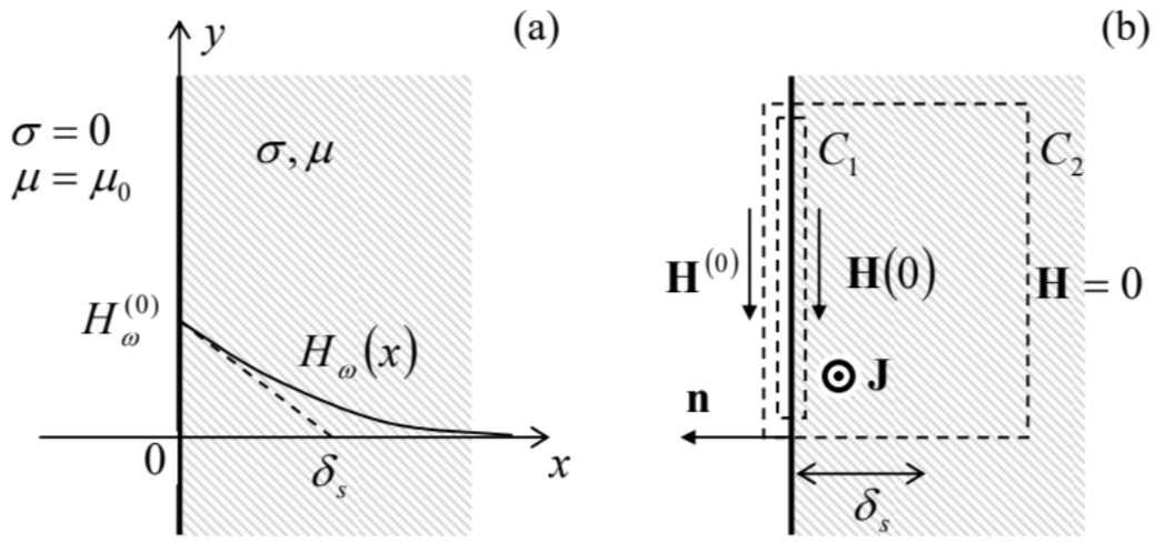
Selecting the coordinate system as shown in Fig. 2a, we may express this condition as
H|x=−0=H(0)(t)ny.
The translational symmetry of our simple problem within the surface plane [y, z] implies that inside the conductor ∂/∂y=∂/∂z=0 as well, and H=H(x,t)ny even at x≥0, so that Eq. (23) for the conductor’s interior is reduced to a differential equation for just one scalar function H(x,t)=B(x,t)/μ:
∂H∂t=1σμ∂2H∂x2, for x≥0.
This equation may be further simplified by noticing that due to its linearity, we may use the linear superposition principle for the time dependence of the field,14 via expanding it, as well as the external field (24), into the Fourier series:
H(x,t)=∑ωHω(x)e−iωt, for x.≥0,H(0)(t)=∑ωH(0)ωe−iωt, for x=−0,
and arguing that if we know the solution for each frequency component of the series, the whole field may be found through the straightforward summation (26) of these solutions.
For each single-frequency component, Eq. (25) is immediately reduced to an ordinary differential equation for the complex amplitude Hω(x):15
−iωHω=1σμd2dx2Hω.
From the theory of linear ordinary differential equations, we know that Eq. (27) has the following general solution:
Hω(x)=H+eκ+x+H−eκ−x,
where the constants κ± are the roots of the characteristic equation that may be obtained by substitution of any of these two exponents into the initial differential equation. For our particular case, the characteristic equation, following from Eq. (27), is
−iω=κ2σμ
and its roots are complex constants
κ±=(−iμωσ)1/2≡±1−i√2(μωσ)1/2.
For our problem, the field cannot grow exponentially at x→+∞, so that only one of the coefficients, namely H_ corresponding to the decaying exponent, with Re κ<0 (i.e. κ=κ−), may be different from zero, i.e. Hω(x)=Hω(0)exp{κ−x}. To find the constant factor Hω(0), we can integrate the macroscopic Maxwell equation ∇×H=j along a pre-surface contour – say, the contour C1 shown in Fig. 2b. The right-hand side’s integral is negligible because the stand-alone current density j does not include the “genuinely-surface” currents responsible for the magnetic permeability μ – see Fig. 5.12. As a result, we get the boundary condition similar to Eq. (5.117) for the stationary magnetic field: Hτ=const at x=0, i.e.
H(0,t)=H(0)(t), i.e. Hω(0)=H(0)ω,
so that the final solution of our problem may be represented as
Hω(x)=H(0)ωexp{−xδs}exp{−i(ωt−xδs)},
where the constant δs_, with the dimension of length, is called the skin depth:
δs≡−1Reκ−=(2μσω)1/2.Skin depth
This solution describes the skin effect: the penetration of the ac magnetic field, and the eddy currents j, into a conductor only to a finite depth of the order of δs.16 Let me give a few numerical examples of this depth: for copper at room temperature, δs≈1 cm at the ac power distribution frequency of 60 Hz, and is of the order of just 1 μm at a few GHz, i.e. at typical frequencies of cell phone signals and kitchen microwave magnetrons. On the other hand, for lightly salted water, δs is close to 250 m at just 1 Hz (with significant implications for radio communications with submarines), and of the order of 1 cm at a few GHz (explaining, in particular, nonuniform heating of a soup bowl in a microwave oven).
In order to complete the skin effect discussion, let us consider what happens with the induced eddy currents17 and the electric field at this effect. When deriving our basic equation (23), we have used, in particular, relations j=∇×H=∇×B/μ, and E=j/σ. Since a spatial differentiation of an exponent yields a similar exponent, the electric field and current density have the same spatial dependence as the magnetic field, i.e. penetrate inside the conductor only by distances of the order of δs(ω), but their vectors are directed perpendicularly to B, while still being parallel to the conductor’s surface:
jω(x)=κ−Hω(x)nz,Eω(x)=κ−σHω(x)nz.
We may use these expressions to calculate the time-averaged power density (4.39) of the energy dissipation, for the important case of a sinusoidal (“monochromatic”) field H(x,t)=|Hω(x)|cos(ωt+φ), and hence sinusoidal eddy currents: j(x,t)=|jω(x)|cos(ωt+φ′):
ˉI(x)=¯j2(x,t)σ=|jω(x)|2¯cos2(ωt+φ′)σ=|jω(x)|22σ=|κ−|2|Hω(x)|22σ=|Hω(x)|2δ2sσ≡Hω(x)H∗ω(x)δ2sσ.
Now the (elementary) integration of this expression along the x-axis (through all the skin depth), using the exponential law (6.32), gives us the following average power of the energy loss per unit area:
Energy loss at skin effectd¯PdA≡∫∞0ˉI(x)dx=12δsσ|H(0)ω|2≡μωδs4|H(0)ω|2.
We will extensively use this expression in the next chapter to calculate the energy losses in microwave waveguides and resonators with conducting (practically, metallic) walls, and for now let us note only that according to Eqs. (33) and (36), for a fixed magnetic field amplitude, the losses grow with frequency as ω1/2.
One more important remark concerning Eqs. (34): integrating the first of them over x, with the help of Eq. (32), we may see that the linear density J of the surface currents (measured in A/m), is simply and fundamentally related to the applied magnetic field:
Jω≡∫∞0jω(x)dx=H(0)ωnz.
Since this relation does not have any frequency-dependent factors, we may sum it up for all frequency components, and get a universal relation
J(t)=H(0)(t)nz≡H(0)(t)(−ny×nx)=H(0)(t)×(−nx)=H(0)(t)×n,
(where n=−nx is the outer normal to the surface – see Fig. 2b) or, in a different form,
ΔH(t)=n×J(t),Coarse-grain boundary relation
where ΔH is the full change of the field through the skin layer. This simple coarse-grain relation (independent of the choice of coordinate axes), is independent of the used constituent relations (22), and is by no means occasional. Indeed, it may be readily obtained from the macroscopic Ampère law (5.116), applied to a contour drawn around a fragment of the surface, extending under it substantially deeper than the skin depth – see the contour C2 in Fig. 2b, and is valid regardless of the exact law of the field penetration.
For the skin effect, this fundamental relationship between the linear current density and the external magnetic field implies that the skin effect’s implementation does not necessarily require a dedicated ac magnetic field source. For example, the effect takes place in any wire that carries an ac current, leading to a current’s concentration in a surface sheet of thickness ∼δs. (Of course, the quantitative analysis of this problem in a wire with an arbitrary cross-section may be technically complicated, because it requires solving Eq. (23) for a 2D geometry; even for the round cross-section, the solution involves the Bessel functions – see Problem 9.) In this case, the ac magnetic field outside the conductor, which still obeys Eq. (38), may be better interpreted as the effect, rather than the reason, of the ac current flow.
Finally, please mind the limited validity of all the above results. First, for the quasistatic approximation to be valid, the field frequency ω should not be too high, so that the displacement current effects are negligible. (Again, this condition will be quantified in Sec. 7 below; it will show that for metals, the condition is violated only at extremely high frequencies above ∼1018 s−1.) A more practical upper limit on ω is that the skin depth δs should stay much larger than the mean free path l of charge carriers,18 because beyond this point, the relation between the vectors j(r) and E(r) becomes essentially non-local. Both theory and experiment show that at δs below l, the skin effect persists, but acquires a frequency dependence slightly different from Eq. (33): δs∝ω−1/3 rather than ω−1/2. This so-called anomalous skin effect has useful applications, for example, for experimental measurements of the Fermi surface of metals.19
Reference
11 Obviously, in free space the last replacement is unnecessary, because all charges and currents may be treated as “stand-alone” ones.
12 See, e.g., MA Eq. (11.3).
13 Due to the simple linear relation B=μH between the fields B and H, it does not matter too much which of
them is used for the solution of this problem, with a slight preference for H, due to the simplicity of Eq. (5.117) – the only boundary condition relevant for this simple geometry.
14 Another important way to exploit the linearity of Eq. (6.25) is to use the spatial-temporal Green’s function approach to explore the dependence of its solutions on various initial conditions. Unfortunately, because of lack of time, I have to leave an analysis of this opportunity for the reader’s exercise.
15 Let me hope that the reader is not intimidated by the (very convenient) use of such complex variables for describing real fields; their imaginary parts always disappear at the final summation (26). For example, if the external field is purely sinusoidal, with the actual (positive) frequency ω, each sum in Eq. (26) has just two terms, with complex amplitudes Hω and H−ω=H∗ω, so that their sum is always real. (For a more detailed discussion of this issue, see, e.g., CM Sec. 5.1.)
16 Let me hope that the physical intuition of the reader makes it evident that the ac field penetrates into a sample of any shape by a similar distance.
17 The loop (vortex) character of the induced current lines, responsible for the term “eddy”, is not very apparent in the 1D geometry explored above, with the near-surface currents (Fig. 2b) looping only implicitly, at z→±∞.
18 A brief discussion of the mean free path may be found, for example, in SM Chapter 6. In very clean metals at very low temperatures, δs may approach l at frequencies as low as ~1 GHz, but at room temperature, the crossover from the normal to the anomalous skin effect takes place only at ~ 100 GHz.
19 See, e.g., A. Abrikosov, Introduction to the Theory of Normal Metals, Academic Press, 1972.