6.5: Electrodynamics of Macroscopic Quantum Phenomena

Despite the superficial similarity of the skin effect and the Meissner-Ochsenfeld effect, the electrodynamics of superconductors is much richer. For example, let us use Eq. (54) to describe the fascinating effect of magnetic flux quantization. Consider a closed ring/loop (not necessarily round one) made of a superconducting “wire” with a cross-section much larger than \(\ \delta_{\mathrm{L}}^{2}\) (Fig. 4a).

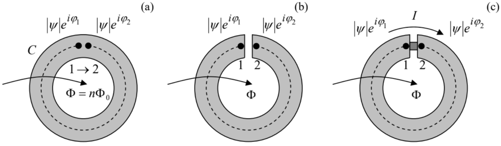Fig. 6.4. (a) A closed, flux-quantizing superconducting ring, (b) a ring with a narrow slit, and (c) a Superconducting QUantum Interference Device (SQUID).

From the last section’s discussion, we know that deep inside the wire the supercurrent is exponentially small. Integrating Eq. (54) along any closed contour C that does not approach the surface closer than a few \(\ \delta_{\mathrm{L}}\) at any point (see the dashed line in Fig. 4), so that with \(\ \mathbf{j}=0\) at all its points, we get

\[\ \oint_{C} \nabla \varphi \cdot d \mathbf{r}-\frac{q}{\hbar} \oint_{C} \mathbf{A} \cdot d \mathbf{r}=0.\tag{6.60}\]

The first integral, i.e. the difference of \(\ \varphi\) in the initial and final points, has to be equal to either zero or an integer number of \(\ 2 \pi\), because the change \(\ \varphi \rightarrow \varphi+2 \pi n\) does not change the Cooper pair’s condensate’s wavefunction:

\[\ \psi^{\prime} \equiv|\psi| e^{i(\varphi+2 \pi n)}=|\psi| e^{i \varphi} \equiv \psi.\tag{6.61}\]

On the other hand, according to Eq. (5.65), the second integral in Eq. (60) is just the magnetic flux \(\ \Phi\) through the contour.³² As a result, we get a wonderful result:

\[\ \text{Magnetic flux quantization}\quad\quad\quad\quad\Phi=n \Phi_{0}, \quad \text { where } \Phi_{0} \equiv \frac{2 \pi \hbar}{|q|}, \quad \text { with } n=0, \pm 1, \pm 2, \ldots,\tag{6.62}\]

saying that the magnetic flux inside any superconducting loop can only take values multiple of the flux quantum \(\ \Phi_{0}\). This effect, predicted in 1950 by the same Fritz London (who expected \(\ q\) to be equal to the electron charge \(\ -e\)), was confirmed experimentally in 1961,³³ but with \(\ |q|=2 e\) - so that \(\ \Phi_{0} \approx 2.07 \times 10^{-15}\) Wb. Historically, this observation gave decisive support to the BSC theory of superconductivity, implying Cooper pairs with charge \(\ q=-2 e\), which had been put forward just four years before.

Note the truly macroscopic character of this quantum effect: it has been repeatedly observed in human-scale superconducting loops, and from what is known about superconductors, there is no doubt that if we have made a giant superconducting wire loop extending, say, over the Earth’s equator, the magnetic flux through it would still be quantized – though with a very large flux quanta number \(\ n\). This means that the quantum coherence of Bose-Einstein condensates may extend over, using H. Casimir’s famous expression, “miles of dirty lead wire”. (Lead is a typical superconductor, with \(\ T_{\mathrm{c}} \approx 7.2 \mathrm{~K}\), and indeed retains its superconductivity even being highly contaminated by impurities.)

Moreover, hollow rings are not entirely necessary for flux quantization. In 1957, A. Abrikosov explained the counter-intuitive high-field behavior of superconductors with \(\ \delta_{\mathrm{L}}>\xi \sqrt{2}\), known experimentally as their mixed (or “Shubnikov”) phase since the 1930s. He showed that a sufficiently high magnetic field may penetrate such superconductors in the form of self-formed magnetic field “threads” (or “tubes”) surrounded by vortex-shaped supercurrents – the so-called Abrikosov vortices. In the simplest case, the core of such a vortex is a straight line, on which the superconductivity is completely suppressed \(\ (|\psi|=0)\), surrounded by circular, axially-symmetric, persistent supercurrents \(\ \mathbf{j}(\rho)\), where \(\ \rho\) is the distance from the vortex axis – see Fig. 5a. At the axis, the current vanishes, and with the growth of \(\ \rho\), it first rises and then falls (with \(\ \mathbf{j}(\infty)=0\)), reaching its maximum at \(\ \rho \sim \xi\), while the magnetic field \(\ \mathbf{B}(\rho)\), directed along the vortex axis, is largest at \(\ \rho=0\), and drops monotonically at distances of the order of \(\ \delta_ \mathrm{L}\) (Fig. 5b).

Fig. 6.5. The Abrikosov vortex: (a) a 3D structure’s sketch, and (b) the main variables as functions of the distance \(\ \rho\) from the axis (schematically).

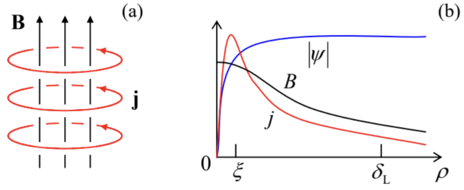
The total flux of the field equals exactly one flux quantum \(\ \Phi_{0}\), given by Eq. (62). Correspondingly, the wavefunction’s phase \(\ \varphi\) performs just one \(\ \pm 2 \pi\) revolution along any contour drawn around the vortex’s axis, so that \(\ \nabla \varphi=\pm \mathbf{n}_{\varphi} /\rho\), where \(\ \mathbf{n}_{\varphi}\) is the azimuthal unit vector.³⁴ This topological feature of the wavefunction’s phase is sometimes called the fluxoid quantization – to distinguish it from the magnetic flux quantization, which is valid only for relatively large contours, not approaching the axis by distances \(\ \sim \delta_{\mathrm{L}}\).

A quantitative analysis of Abrikosov vortices requires, besides the equations we have discussed, one more constituent equation that would describe the suppression of the number of Cooper pairs (quantified by \(\ |\psi|^{2}\)) by the magnetic field – or rather by the field-induced supercurrent. In his original work, Abrikosov used for this purpose the famous Ginzburg-Landau equation,³⁵ which is quantitatively valid only at \(\ T \approx T_{\mathrm{c}}\). The equation may be conveniently represented using either of the following two forms:

\[\ \frac{1}{2 m}(-i \hbar \nabla-q \mathbf{A})^{2} \psi=a \psi-b \psi|\psi|^{2}, \quad \xi^{2} \psi *\left(\nabla-i \frac{q}{\hbar} \mathbf{A}\right)^{2} \psi=\left(1-|\psi|^{2}\right)|\psi|^{2},\tag{6.63}\]

where \(\ a\) and \(\ b\) are certain temperature-dependent coefficients, with \(\ a \rightarrow 0\) at \(\ T \rightarrow T_{\mathrm{c}}\). The first of these forms clearly shows that the Ginzburg-Landau equation (as well as the similar Gross-Pitaevskii equation describing uncharged Bose-Einstein condensates) belongs to a broader class of nonlinear Schrödinger equations, differing only by the additional nonlinear term from the usual Schrödinger equation, which is linear in \(\ \psi\). The equivalent, second form of Eq. (63) is more convenient for applications, and shows more clearly that if the superconductor’s condensate density, proportional to \(\ |\psi|^{2}\), is suppressed only locally, it self-restores to its unperturbed value (with \(\ |\psi|^{2}=1\)) at the distances of the order of the coherence length \(\ \xi \equiv \hbar /(2 m a)^{1 / 2}\).

This fact enables a simple quantitative analysis of the Abrikosov vortex in the most important limit \(\ \xi<<\delta_{\mathrm{L}}\). Indeed, in this case (see Fig. 5) \(\ |\psi|^{2}=1\) at most distances \(\ \left(\rho \sim \delta_{\mathrm{L}}\right)\) where the field and current are distributed, so that these distributions may be readily calculated without any further involvement of Eq. (63), just from Eq. (54) with \(\ \nabla \varphi=\pm \mathbf{n}_{\varphi} /\rho\), and the Maxwell equations (21) for the
magnetic field, giving \(\ \nabla \times \mathbf{B}=\mu \mathbf{j}\), and \(\ \nabla \cdot \mathbf{B}=0\). Indeed, combining these equations just as this was done at the derivation of Eq. (23), for the only Cartesian component of the vector \(\ \mathbf{B}(\mathbf{r})=B(\rho) \mathbf{n}_{z}\) (where the z-axis is directed along the vortex’ axis), we get a simple equation

\[\ \delta_{\mathrm{L}}^{2} \nabla^{2} B-B=-\frac{\hbar}{q} \nabla \times(\nabla \times \varphi) \equiv \mp \Phi_{0} \delta_{2}(\mathbf{\rho}), \quad \text { at } \rho>>\xi,\tag{6.64}\]

which coincides with Eq. (56) at all regular points \(\ \rho \neq 0\), Spelling out the Laplace operator for our current case of axial symmetry,³⁶ we get an ordinary differential equation,

\[\ \delta_{\mathrm{L}}^{2} \frac{1}{\rho} \frac{d}{d \rho}\left(\rho \frac{d B}{d \rho}\right)-B=0, \quad \text { for } \rho \neq 0.\tag{6.65}\]

Comparing this equation with Eq. (2.155) with \(\ \nu=0\), and taking into account that we need the solution decreasing at \(\ \rho \rightarrow \infty\), making any contribution proportional to the function \(\ I_{0}\) unacceptable, we get

\[\ B=C K_{0}\left(\frac{\rho}{\delta_{\mathrm{L}}}\right)\tag{6.66}\]

- see the plot of this function (black line) on the right panel of Fig. 2.22. The constant \(\ C\) should be calculated from fitting the 2D delta function on the right-hand side of Eq. (64), i.e. by requiring

\[\ \int_{\text {vortex }} B(\rho) d^{2} \rho \equiv 2 \pi \int_{0}^{\infty} B(\rho) \rho d \rho \equiv 2 \pi \delta_{\mathrm{L}}^{2} C \int_{0}^{\infty} K_{0}(\zeta) \zeta d \zeta=\mp \Phi_{0}.\tag{6.67}\]

The last, dimensionless integral equals 1,³⁷ so that finally

\[\ B(\rho)=\frac{\Phi_{0}}{2 \pi \delta_{\mathrm{L}}^{2}} K_{0}\left(\frac{\rho}{\delta_{\mathrm{L}}}\right), \quad \text { at } \rho>>\xi.\tag{6.68}\]

Function \(\ K_{0}\) (the modified Bessel function of the second kind), drops exponentially as its argument becomes larger than 1 (i.e., in our problem, at distances \(\ \rho\) much larger than \(\ \delta_{\mathrm{L}}\)), and diverges as its argument tends to zero – see, e.g., the second of Eqs. (2.157). However, this divergence is very slow (logarithmic), and, as was repeatedly discussed in this series, is avoided by the account of virtually any other factor. In our current case, this factor is the decrease of \(\ |\psi|^{2}\) to zero at \(\ \rho \sim \xi\) (see Fig. 5), not taken into account in Eq. (68). As a result, we may estimate the field on the axis of the vortex as

\[\ B(0) \approx \frac{\Phi_{0}}{2 \pi \delta_{\mathrm{L}}^{2}} \ln \frac{\delta_{\mathrm{L}}}{\xi};\tag{6.69}\]

the exact (and much more involved) solution of the problem confirms this estimate with a minor correction: \(\ \ln \left(\delta_{\mathrm{L}} / \xi\right) \rightarrow \ln \left(\delta_{\mathrm{L}} / \xi\right)-0.28\).

The current density distribution may be now calculated from the Maxwell equation \(\ \nabla \times \mathbf{B}=\mu \mathbf{j}\), giving \(\ \mathbf{j}=j(\rho) \mathbf{n}_{\varphi}\), with³⁸

\[\ j(\rho)=-\frac{1}{\mu} \frac{\partial B}{\partial \rho}=-\frac{\Phi_{0}}{2 \pi \mu \delta_{\mathrm{L}}^{2}} \frac{\partial}{\partial \rho} K_{0}\left(\frac{\rho}{\delta_{\mathrm{L}}}\right) \equiv \frac{\Phi_{0}}{2 \pi \mu \delta_{\mathrm{L}}^{3}} K_{1}\left(\frac{\rho}{\delta_{\mathrm{L}}}\right), \quad \text { at } \rho>>\xi,\tag{6.70}\]

where the same identity (2.158), with \(\ J_{n} \rightarrow K_{n}\), and \(\ n=1\), was used. Now looking at Eqs. (2.157) and (2.158), with \(\ n = 1\), we see that the supercurrent’s density is exponentially low at \(\ \rho >> \delta_{\mathrm{L}}\) (thus outlining the vortex’ periphery), and is proportional to \(\ 1 / \rho\) within the broad range \(\ \xi<<\rho<<\delta_{\mathrm{L}}\). This rise of the current at \(\ \rho \rightarrow 0\) (which could be readily predicted directly from Eq. (54) with \(\ \nabla \varphi=\pm \mathbf{n}_{\varphi} /\rho\), and the \(\ \mathbf{A}\)-term negligible at \(\ \rho<<\delta_{\mathrm{L}}\)) is quenched at \(\ \rho \sim \xi\) by a rapid drop of the factor \(\ |\psi|^{2}\) in the same Eq. (54), i.e. by the suppression of the superconductivity near the axis (by the same supercurrent!) – see Fig. 5 again.

This vortex structure may be used to calculate, in a straightforward way, its energy per unit length (i.e. its linear tension)

\[\ \mathscr{T} \equiv \frac{U}{l} \approx \frac{\Phi_{0}^{2}}{4 \pi \mu \delta_{\mathrm{L}}^{2}} \ln \frac{\delta_{\mathrm{L}}}{\xi},\tag{6.71}\]

and hence the so-called “first critical” value \(\ H_{\mathrm{cl}}\) of the external magnetic field,³⁹ at that the vortex formation becomes possible (in a long cylindrical sample parallel to the field):

\[\ H_{\mathrm{cl}}=\frac{\mathscr{T}}{\Phi_{0}} \approx \frac{\Phi_{0}}{4 \pi \mu \delta_{\mathrm{L}}^{2}} \ln \frac{\delta_{\mathrm{L}}}{\xi}.\tag{6.72}\]

Let me leave the proof of these two formulas for the reader’s exercise.

The flux quantization and the Abrikosov vortices discussed above are just two of several macroscopic quantum effects in superconductivity. Let me discuss just one more, but perhaps the most interesting of such effects. Let us consider a superconducting ring/loop interrupted with a very narrow slit (Fig. 4b). Integrating Eq. (54) along any current free path from point 1 to point 2 (see, e.g., dashed line in Fig. 4b), we get

\[\ 0=\int_{1}^{2}\left(\nabla \varphi-\frac{q}{\hbar} \mathbf{A}\right) \cdot d \mathbf{r}=\varphi_{2}-\varphi_{1}-\frac{q}{\hbar} \Phi.\tag{6.73}\]

Using the flux quantum definition (62), this result may be rewritten as

\[\ \varphi \equiv \varphi_{1}-\varphi_{2}=\frac{2 \pi}{\Phi_{0}} \Phi,\quad\quad\quad\quad\text{Josephson phase difference}\tag{6.74}\]

where \(\ \varphi\) is called the Josephson phase difference. Note that in contrast to each of the phases \(\ \varphi_{1,2}\), their difference \(\ \varphi\) is gauge-invariant: Eq. (74) directly relates it to the gauge-invariant magnetic flux \(\ \Phi\).

Can this \(\ \varphi\) be measured? Yes, using the Josephson effect.⁴⁰ Let us consider two (for the argument simplicity, similar) superconductors, connected with some sort of weak link, for example, either a tunnel junction, or a point contact, or a narrow thin-film bridge, through that a weak Cooper-pair supercurrent can flow. (Such a system of two weakly coupled superconductors is called a Josephson junction.) Let us think about what this supercurrent \(\ I\) may be a function of. For that, reverse thinking is helpful: let us imagine that we change the current; what parameter of the superconducting condensate can it affect? If the current is weak, it cannot perturb the superconducting condensate’s density, proportional to \(\ |\psi|^{2}\); hence it may only change the Cooper condensate phases \(\ \varphi_{1,2}\). However, according to Eq. (53), the phases are not gauge-invariant, while the current should be. Hence the current may affect (or, if you like, may be affected by) only the phase difference \(\ \varphi\) defined by Eq. (74). Moreover, just has already been argued during the flux quantization discussion, a change of any of \(\ \varphi_{1,2}\) (and hence of \(\ \varphi\)) by \(\ 2 \pi\) or any of its multiples should not change the current. Also, if the wavefunction is the same in both superconductors \(\ (\varphi=0)\), the supercurrent should vanish due to the system’s symmetry. Hence the function \(\ I(\varphi)\) should satisfy the following conditions:

\[\ I(0)=0, \quad I(\varphi+2 \pi)=I(\varphi).\tag{6.75}\]

With these conditions on hand, we should not be terribly surprised by the following Josephson’s result that for the weak link provided by tunneling,⁴¹

\[\ \text{Josephson (super) current}\quad\quad\quad\quad I(\varphi)=I_{\mathrm{c}} \sin \varphi\tag{6.76}\]

where constant \(\ I_{\mathrm{c}}\), which depends on the weak link’s strength and temperature, is called the critical current. Actually, Eqs. (54) and (63) enable not only a straightforward calculation of this relation, but even obtaining a simple expression of the critical current \(\ I_{\mathrm{c}}\) via the link’s normal-sate resistance – the
task left for the (creative :-) reader’s exercise.

Now let us see what happens if a Josephson junction is placed into the gap in a superconductor loop – see Fig. 4c. In this case, we may combine Eqs. (74) and (76), getting

\[\ \text{Macroscopic quantum interference}\quad\quad\quad\quad I=I_{\mathrm{c}} \sin \left(2 \pi \frac{\Phi}{\Phi_{0}}\right).\tag{6.77}\]

This effect of a periodic dependence of the current on the magnetic flux is called the macroscopic quantum interference, ⁴² while the system shown in Fig. 4c, the superconducting quantum interference device – SQUID (with all letters capital, please :-). The low value of the magnetic flux quantum \(\ \Phi_{0}\), and hence the high sensitivity of \(\ \varphi\) to external magnetic fields, allows using such SQUIDs as ultrasensitive magnetometers. Indeed, for a superconducting ring of area \(\ \sim 1 \mathrm{~cm}^{2}\), one period of the change of the supercurrent (77) is produced by a magnetic field change of the order of \(\ 10^{-11} \mathrm{~T}\left(10^{-7} \mathrm{Gs}\right)\), while sensitive electronics allows measuring a tiny fraction of this period – limited by thermal noise at a level of the order of a few fT. Such sensitivity allows measurements, for example, of the magnetic fields induced outside of the body by the beating human heart, and even by the brain activity.⁴³

An important aspect of quantum interference is the so-called Aharonov-Bohm (AB) effect (which actually takes place for single quantum particles as well).⁴⁴ Let the magnetic field lines be limited to the central part of the SQUID ring, so that no appreciable magnetic field ever touches the superconducting ring. (This may be done experimentally with very good accuracy, for example using high-\(\ \mu\) magnetic cores – see their discussion in Sec. 5.6.) As predicted by Eq. (77), and confirmed by several careful experiments carried out in the mid-1960s,⁴⁵ this restriction does not matter – the interference is observed anyway. This means that not only the magnetic field \(\ \mathbf{B}\) but also the vector potential \(\ \mathbf{A}\) represents physical reality, albeit in a quite peculiar way – remember the gauge transformation (5.46), which you may carry out in the top of your head, without changing any physical reality? (Fortunately, this transformation does not change the contour integral participating in Eq. (5.65), and hence the magnetic flux \(\ \text { Ф }\), and hence the interference pattern.)

Actually, the magnetic flux quantization (62) and the macroscopic quantum interference (77) are not completely different effects, but just two manifestations of the interrelated macroscopic quantum phenomena. To show that, one should note that if the critical current \(\ I_{\mathrm{c}}\) (or rather its product by the loop’s self-inductance \(\ L\)) is high enough, the flux \(\ \Phi\) in the SQUID loop is due not only to the external magnetic field flux \(\ \Phi_{\mathrm{ext}}\) but also has a self-field component – cf. Eq. (5.68):⁴⁶

\[\ \Phi=\Phi_{\mathrm{ext}}-L I, \quad \text { where } \Phi_{\mathrm{ext}} \equiv \int_{S}\left(B_{\mathrm{ext}}\right)_{n} d^{2} r.\tag{6.78}\]

Now the relation between \(\ \Phi\) and \(\ \Phi_{\mathrm{ext}}\) may be readily found by solving this equation together with Eq. (77). Figure 6 shows this relation for several values of the dimensionless parameter \(\ \lambda \equiv 2 \pi L I_{\mathrm{c}} / \Phi_{0}\).

Fig. 6.6. The function \(\ \Phi\left(\Phi_{\text {ext }}\right)\) for SQUIDs with various values of the normalized \(\ L I_{\mathrm{c}}\) product. Dashed arrows show the flux leaps as the external field is changed. (The branches with \(\ d \Phi / d \Phi_{\text {ext }}<0\) are unstable.)

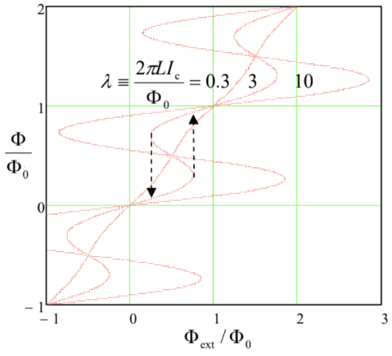
These plots show that if the critical current (and/or the inductance) is low, \(\ \lambda<<1\), the self-field effects are negligible, and the total flux follows the external field (i.e., \(\ \Phi_{\text {ext }}\)) faithfully. However, at \(\ \lambda>1\), the function \(\ \Phi\left(\Phi_{\text {ext }}\right)\) becomes hysteretic, and at \(\ \lambda >> 1\) the stable (positive-slope) branches of this function are nearly flat, with the total flux values corresponding to Eq. (62). Thus, a superconducting ring closed with a high-\(\ I_{\mathrm{c}}\) Josephson junction exhibits a nearly-perfect flux quantization.

The self-field effects described by Eq. (78) create certain technical problems for SQUID magnetometry, but they are the basis for one more useful application of these devices: ultrafast computing. Indeed, Fig. 6 shows that at the values of \(\ \lambda\) modestly above 1 (e.g., \(\ \lambda \approx 3\)), and within a certain range of applied field, the SQUID has two stable flux states that differ by \(\ \Delta \Phi \approx \Phi_{0}\) and may be used for coding binary 0 and 1. For practical superconductors (like Nb), the time of switching between these states (see dashed arrows in Fig. 4) is of the order of a picosecond, while the energy dissipated at such event may be as low as \(\ \sim 10^{-19} \mathrm{~J}\). (This bound is determined not by device’s physics, by the fundamental requirement for the energy barrier between the two states to be much higher than the thermal fluctuation energy scale \(\ k_{\mathrm{B}} T\), ensuring a sufficiently long information retention time.) While the picosecond switching speed may be also achieved with some semiconductor devices, the power consumption of the SQUID-based digital devices may be 5 to 6 orders of magnitude lower, enabling VLSI integrated circuits with 100-GHz-scale clock frequencies. Unfortunately, the range of practical applications of these Rapid Single-Flux-Quantum (RSFQ) digital circuits is still very narrow, due to the inconvenience of their deep refrigeration to temperatures below \(\ T_{\mathrm{c}}\).⁴⁷

Since we have already got the basic relations (74) and (76) describing the macroscopic quantum phenomena in superconductivity, let me mention in brief two other members of this group, called the dc and ac Josephson effects. Differentiating Eq. (74) over time, and using the Faraday induction law (2), we get⁴⁸

\[\ \text{Josephson phase-to-voltage relation}\quad\quad\quad\quad\frac{d \varphi}{d t}=\frac{2 e}{\hbar} V\tag{6.79}\]

This famous Josephson phase-to-voltage relation should be valid regardless of the way how the voltage \(\ V\) has been created,⁴⁹ so let us apply Eqs. (76) and (79) to the simplest circuit with a non-superconducting source of dc voltage – see Fig. 7.

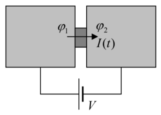Fig. 6.7. DC-voltage-biased Josephson junction.

If the current’s magnitude is below the critical value, Eq. (76) allows the phase \(\ \varphi\) to have the time-independent value

\[\ \varphi=\sin ^{-1} \frac{I}{I_{\mathrm{c}}}, \quad \text { if }-I_{\mathrm{c}}<I<+I_{\mathrm{c}},\tag{6.80}\]

and hence, according to Eq. (79), a vanishing voltage drop across the junction: \(\ V=0\). This dc Josephson effect is not quite surprising – indeed, we have postulated from the very beginning that the Josephson junction may pass a certain supercurrent. Much more fascinating is the so-called ac Josephson effect that occurs if the voltage across the junction has a non-zero average (dc) component \(\ V_{0}\). For simplicity, let us assume that this is the only voltage component: \(\ V(t)=V_{0}=\text { const }\);⁵⁰ then Eq. (79) may be easily integrated to give \(\ \varphi=\omega_{\mathrm{J}} t+\varphi_{0}\), where

\[\ \omega_{\mathrm{J}} \equiv \frac{2 e}{\hbar} V_{0}.\quad\quad\quad\quad\text{Josephson oscillation frequency}\tag{6.81}\]

This result, plugged into Eq. (76), shows that the supercurrent oscillates,

\[\ I=I_{\mathrm{c}} \sin \left(\omega_{\mathrm{J}} t+\varphi_{0}\right),\tag{6.82}\]

with the so-called Josephson frequency \(\ \omega_{\mathrm{J}}\) (81) proportional to the applied dc voltage. For practicable voltages (above the typical noise level), the frequency \(\ f_{\mathrm{J}}=\omega_{\mathrm{J}} / 2 \pi\) corresponds to the GHz or even THz ranges, because the proportionality coefficient in Eq. (81) is very high: \(\ f_{\mathrm{J}} / V_{0}=e / \pi \hbar \approx 483 \mathrm{MHz} / \mu \mathrm{V}\).⁵¹

An important experimental fact is the universality of this coefficient. For example, in the mid-1980s, a Stony Brook group led by J. Lukens proved that this factor is material independent with the relative accuracy of at least \(\ 10^{-15}\). Very few experiments, especially in solid-state physics, have ever reached such precision. This fundamental nature of the Josephson voltage-to-frequency relation (81) allows an important application of the ac Josephson effect in metrology. Namely, phase-locking⁵² the Josephson oscillations with an external microwave signal from an atomic frequency standard, one can get a more precise dc voltage than from any other source. In NIST, and other metrological institutions around the globe, this effect is used for calibration of simpler “secondary” voltage standards that can operate at room temperature.

---

Reference

³¹ The material of this section is not covered in most E&M textbooks, and will not be used in later sections of this course. Thus the “only” loss due to the reader’s skipping this section would be the lack of familiarity with one of the most fascinating fields of physics. Note also that we already have virtually all formal tools necessary for its discussion, so that reading this section should not require much effort.

³² Due to the Meissner-Ochsenfeld effect, the exact path of the contour is not important, and we may discuss \(\ \Phi\) just as the magnetic flux through the ring.

³³ Independently and virtually simultaneously by two groups: B. Deaver and W. Fairbank, and R. Doll and M. Näbauer; their reports were published back-to-back in the same issue of the Physical Review Letters.

³⁴ The last (perhaps, evident) expression formally follows from MA Eq. (10.2) with \(\ f=\pm \varphi+\mathrm{const}\).

³⁵ This equation was derived by Vitaly Lazarevich Ginzburg and Lev Davidovich Landau from phenomenological arguments in 1950, i.e. before the advent of the “microscopic” BSC theory, and may be used for simple analyses of a broad range of nonlinear effects in superconductors. The Ginzburg-Landau and Gross-Pitaevskii equations will be further discussed in SM Sec. 4.3.

³⁶ See, e.g., MA Eq. (10.3) with \(\ \partial / \partial \varphi=\partial / \partial z=0\).

³⁷ This fact follows, for example, from the integration of both sides of Eq. (2.143) (which is valid for any Bessel functions, including \(\ K_{n}\)) with \(\ n=1\), from 0 to \(\ \infty\), and then using the asymptotic values given by Eqs. (2.157)-(2.158): \(\ K_{1}(\infty)=0\), and \(\ K_{1}(\zeta) \rightarrow 1 / \zeta\) at \(\ \zeta \rightarrow 0\).

³⁸ See, e.g., MA Eq. (10.5), with \(\ f_{\rho}=f_{\varphi}=0\), and \(\ f_{z}=B(\rho)\).

³⁹ This term is used to distinguish \(\ H_{\mathrm{c} 1}\) from the higher “second critical field” \(\ H_{\mathrm{c} 2}\), at which the Abrikosov vortices are pressed to each other so tightly (to distances \(\ d \sim \xi\)) that they merge, and the remains of superconductivity vanish: \(\ \psi \rightarrow 0\). Unfortunately, I do not have time/space to discuss these effects; the interested reader may be referred, for example, to Chapter 5 of M. Tinkham’s monograph cited above.

⁴⁰ It was predicted in 1961 by Brian David Josephson (then a PhD student!) and observed experimentally by several groups soon after that.

⁴¹ For some other types of weak links, the function \(\ I(\varphi)\) may deviate from the sinusoidal form Eq. (76) rather considerably, while still satisfying the general conditions (75).

⁴² The name is due to a deep analogy between this phenomenon and the interference between two coherent waves, to be discussed in detail in Sec. 8.4.

⁴³ Other practical uses of SQUIDs include MRI signal detectors, high-sensitive measurements of magnetic properties of materials, and weak field detection in a broad variety of physical experiments – see, e.g., J. Clarke and A. Braginski (eds.), The SQUID Handbook, vol. II, Wiley, 2006. For a comparison of these devices with other sensitive magnetometers see, e.g., the review collection by A. Grosz et al. (eds.), High Sensitivity Magnetometers, Springer, 2017.

⁴⁴ For a more detailed discussion of the AB effect see, e.g., QM Sec. 3.2.

⁴⁵ Similar experiments have been carried out with single (unpaired) electrons – moving either ballistically, in vacuum, or in “normal” (non-superconducting) conducting rings. In the last case, the effect is much harder to observe that in SQUIDs, because the ring size has to be very small, and temperature very low, to avoid the so-called dephasing effects due to unavoidable interactions of the electrons with their environment – see, e.g., QM Chapter 7.

⁴⁶ The sign before \(\ L I\) would be positive, as in Eq. (5.70), if \(\ I\) was the current flowing into the inductance. However, in order to keep the sign in Eq. (76) intact, \(\ I\) should mean the current flowing into the Josephson junction, i.e. from the inductance, thus changing the sign of the \(\ LI\) term in Eq. (78).

⁴⁷ For more on that technology, see, e.g., the review paper by P. Bunyk et al., Int. J. High Speed Electron. Syst. 11, 257 (2001), and references therein.

⁴⁸ Since the induced e.m.f. \(\ \mathscr{V}_{\text {ind }}\) cannot drop on the superconducting path between the Josephson junction electrodes 1 and 2 (see Fig. 4c), it should be equal to \(\ (-V)\), where \(\ V\) is the voltage across the junction.

⁴⁹ Indeed, it may be also obtained from simple Schrödinger equation arguments – see, e.g., QM Sec. 1.6.

⁵⁰ In experiment, this condition is hard to implement, due to relatively high inductances of the current leads providing the dc voltage supply. However, this technical complication does not affect the main conclusion of the simple analysis described here.

⁵¹ This 1962 prediction (by the same B. Josephson) was confirmed experimentally – first implicitly, by phase-locking of the oscillations with an external oscillator in 1963, and then explicitly, by the direct detection of the emitted microwave radiation in 1967.

⁵² For a discussion of this very important (and general) effect, see, e.g., CM Sec. 5.4.